Uncertainty I + II

POL51

Haley Daarstad

University of California, Davis

August 26, 2026

Late Assignments

CONTACT ME ASAP!! BEFORE FRIDAY @ 6 PM

I will not be taking any late assignments from the first half of class after Sunday

If you used a wavier, please email me the assignment it was used on so I have it in writing

Plan for today

Why are we uncertain?

Sampling

Quantifying uncertainty

Are we sure it’s not zero?

Where things stand

So far: worrying about causality

how can we know the effect of X on Y is not being confounded by something else?

Last bit: how confident are we in our estimates given…

that our estimates are based on samples?

Uncertainty in the wild

The “bounds” in geom_smooth tells us something about how confident we should be in the line:

Uncertainty

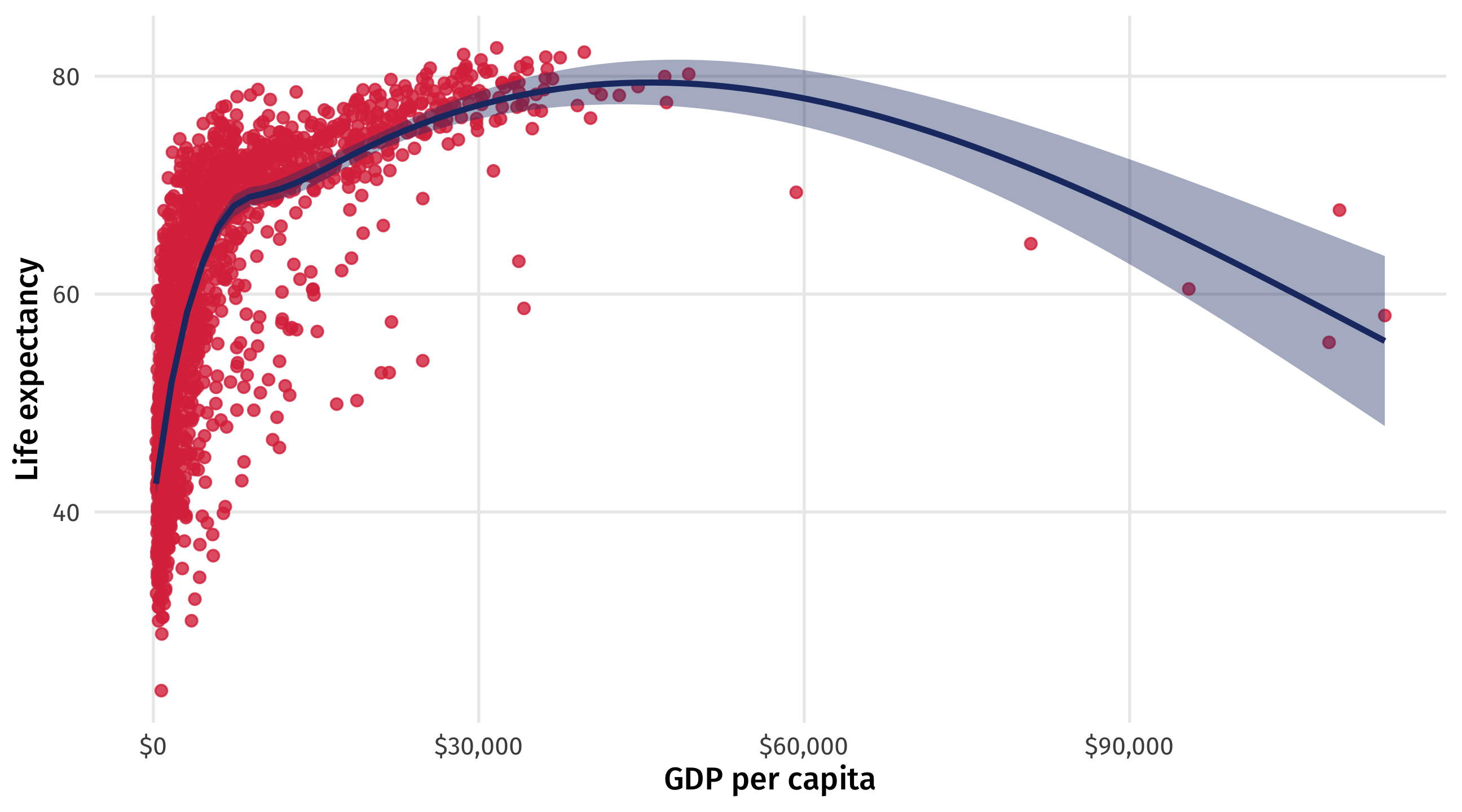
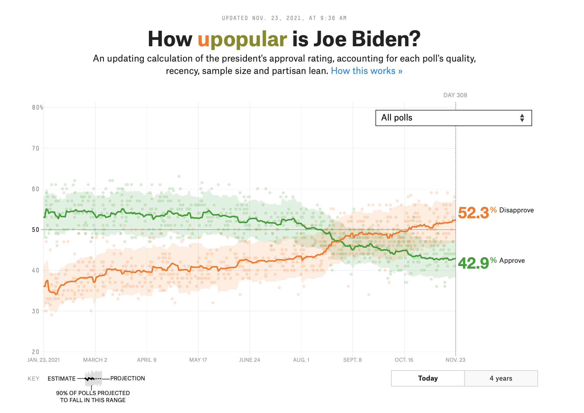
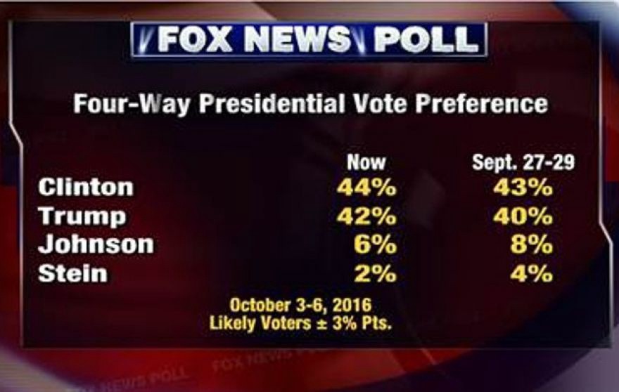
Polling error, margin of error, uncertainty bounds, all help to quantify how uncertain we feel about an estimate

Vague sense that we are uncertain about what we are estimating

But why are we uncertain? And how can uncertainty be quantified?

Why are we uncertain?

We don’t have all the data we care about
We have a sample, such as a survey, or a poll, of a population
Problem each sample will look different, and give us a different answer to the question we are trying to answer

What’s going on here? terminology

Term	Meaning	Example
Population	All of the instances of the thing we care about	American adults
Population parameter	The thing about the population we want to know	Average number of kids among American adults
Sample	A subset of the population	A survey
Sample estimate	Our estimate of the population parameter	Average number of kids in survey

Boring example: kids

How many children does the average American adult have? (Population parameter)

Let’s pretend there were only 2,867 people living in the USA, and they were all perfectly sampled in gss_sm

A few rows from gss_sm
year	age	childs	degree	race	sex
2016	41	3	High School	Black	Male
2016	65	0	High School	Other	Male
2016	27	0	Bachelor	White	Male
2016	49	3	Lt High School	Black	Male
2016	66	2	Lt High School	White	Male

Boring example: kids

How many children does the average American adult have?

We can get the exact answer, since there are only 2,867 Americans, and they’re all in our data:

gss_sm %>% 
  summarise(avg_kids = mean(childs, na.rm = TRUE))

# A tibble: 1 × 1
  avg_kids
     <dbl>
1     1.85

The true average number of children in the US is 1.85 (Population parameter)

Sampling

Now imagine that instead of having data on every American, we only have a sample of 10 Americans

Why do we have a sample? Because interviewing every American is prohibitively costly

Same way a poll works: a sample to estimate American public opinion

Sampling

We can pick one sample of 10 people from gss_sm using the rep_sample_n() function from moderndive:

gss_sm %>% rep_sample_n(size = 10, reps = 1)

# A tibble: 10 × 33
# Groups:   replicate [1]
   replicate  year    id ballot       age childs sibs  degree race  sex   region
       <int> <dbl> <dbl> <labelled> <dbl>  <dbl> <lab> <fct>  <fct> <fct> <fct> 
 1         1  2016   579 2             66      6 14    High … Black Fema… W. So…
 2         1  2016   669 3             27      0  0    High … Black Male  Middl…
 3         1  2016  2185 3             78      4  6    High … White Fema… W. No…
 4         1  2016  2797 3             23      1  7    High … White Fema… E. So…
 5         1  2016  1298 2             52      1  1    Bache… White Fema… W. So…
 6         1  2016   450 2             19      0  0    High … White Fema… New E…
 7         1  2016   431 3             26      0  4    Lt Hi… Other Fema… South…
 8         1  2016  2067 3             52      2  3    High … White Male  E. No…
 9         1  2016  1715 3             41      2  5    Bache… White Fema… South…
10         1  2016  1481 1             57      0  3    Bache… White Fema… E. So…
# ℹ 22 more variables: income16 <fct>, relig <fct>, marital <fct>, padeg <fct>,
#   madeg <fct>, partyid <fct>, polviews <fct>, happy <fct>, partners <fct>,
#   grass <fct>, zodiac <fct>, pres12 <labelled>, wtssall <dbl>,
#   income_rc <fct>, agegrp <fct>, ageq <fct>, siblings <fct>, kids <fct>,
#   religion <fct>, bigregion <fct>, partners_rc <fct>, obama <dbl>

Note

size = size of the sample; reps = number of samples

Sample estimate

We can then calculate the average number of kids among that sample of 10 people

gss_sm %>% rep_sample_n(size = 10, reps = 1) %>% 
  summarise(avg_kids = mean(childs, na.rm = TRUE))

# A tibble: 1 × 2
  replicate avg_kids
      <int>    <dbl>
1         1      1.1

this is our sample estimate of the population parameter

Notice that it does not equal the true population parameter (1.87)

The trouble with samples

Problem: each sample will give you a different estimate. Instead of taking 1 sample of size 10, let’s take 1,000 samples of size 10:

kids_10 = gss_sm %>% rep_sample_n(size = 10, reps = 1000) %>% 
  summarise(avg_kids = mean(childs, na.rm = TRUE))
kids_10

# A tibble: 1,000 × 2
   replicate avg_kids
       <int>    <dbl>
 1         1      1.9
 2         2      1.9
 3         3      1.7
 4         4      1.7
 5         5      2.1
 6         6      2  
 7         7      2.4
 8         8      2.2
 9         9      2.3
10        10      2.2
# ℹ 990 more rows

The trouble with samples

Across 1,000 samples of 10 people each, the estimated average number of kids can vary between 0.2 and 4.2!! Remember, the true average is 1.85

Why are we uncertain?

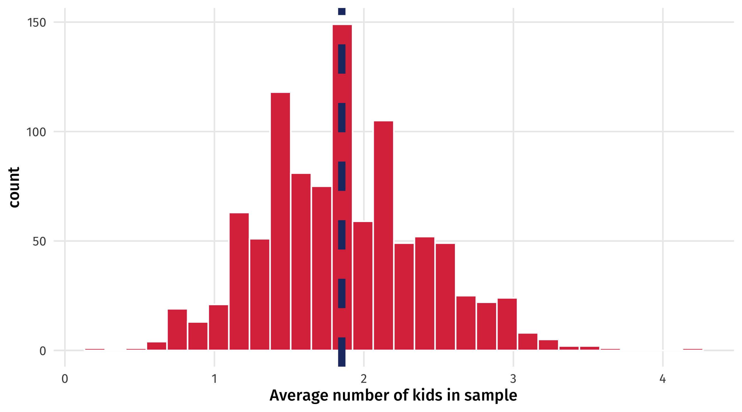
We only ever have a sample (10 random Americans), but we’re interested in something bigger: a population (the whole of gss_sm)

Polls often ask a couple thousand people (if that!), and try to infer something bigger (how all Americans feel about the President)

The problem: Each sample is going to give us different results!

Especially worrisome: some estimates will be way off, totally by chance

A problem for regression

This is also a problem for regression, since every regression estimate is based on a sample

What’s the relationship between sex and vote choice among American voters?

mod1 = lm(obama ~ sex, data = gss_sm)
tidy(mod1)

# A tibble: 2 × 5
  term        estimate std.error statistic   p.value
  <chr>          <dbl>     <dbl>     <dbl>     <dbl>
1 (Intercept)   0.576     0.0177     32.6  5.84e-182
2 sexFemale     0.0871    0.0234      3.72 2.06e-  4

So females were 8.7 percent more likely to vote for Obama than males

This is the population parameter, since we’re pretending all Americans are in gss_sm

Regression estimates vary too

Each sample will produce different regression estimates

replicate	term	estimate
1	sexFemale	0.20
2	sexFemale	-0.11
3	sexFemale	-0.14
4	sexFemale	0.10
5	sexFemale	0.32
6	sexFemale	-0.20
7	sexFemale	0.03
8	sexFemale	-0.13

Wrong effect estimates

Many of the effects we estimate below are even negative! This is the opposite of the population parameter (0.087)

The solution

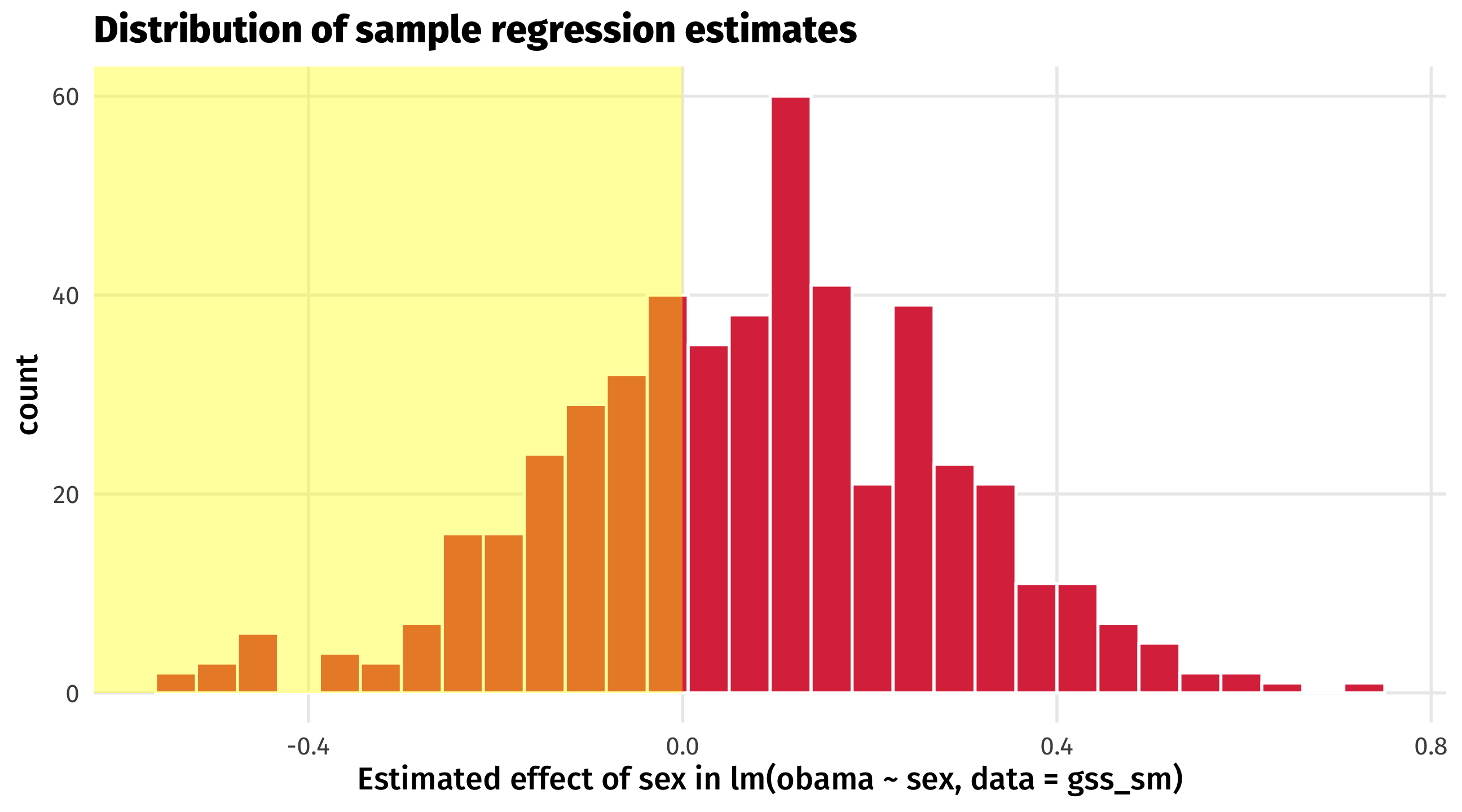
So how do we know if our sample estimate is close to the population parameter?
Turns out that if a sample is random, representative, and large…
…then the LAW OF LARGE NUMBERS tells us that…
the sample estimate will be pretty close to the population parameter

Law of large numbers

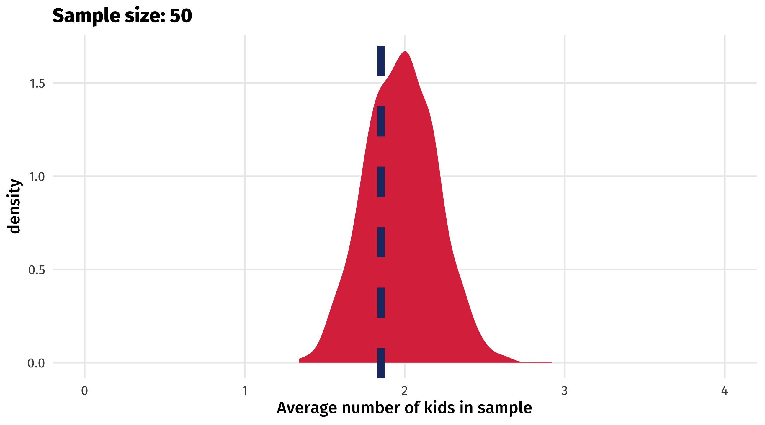
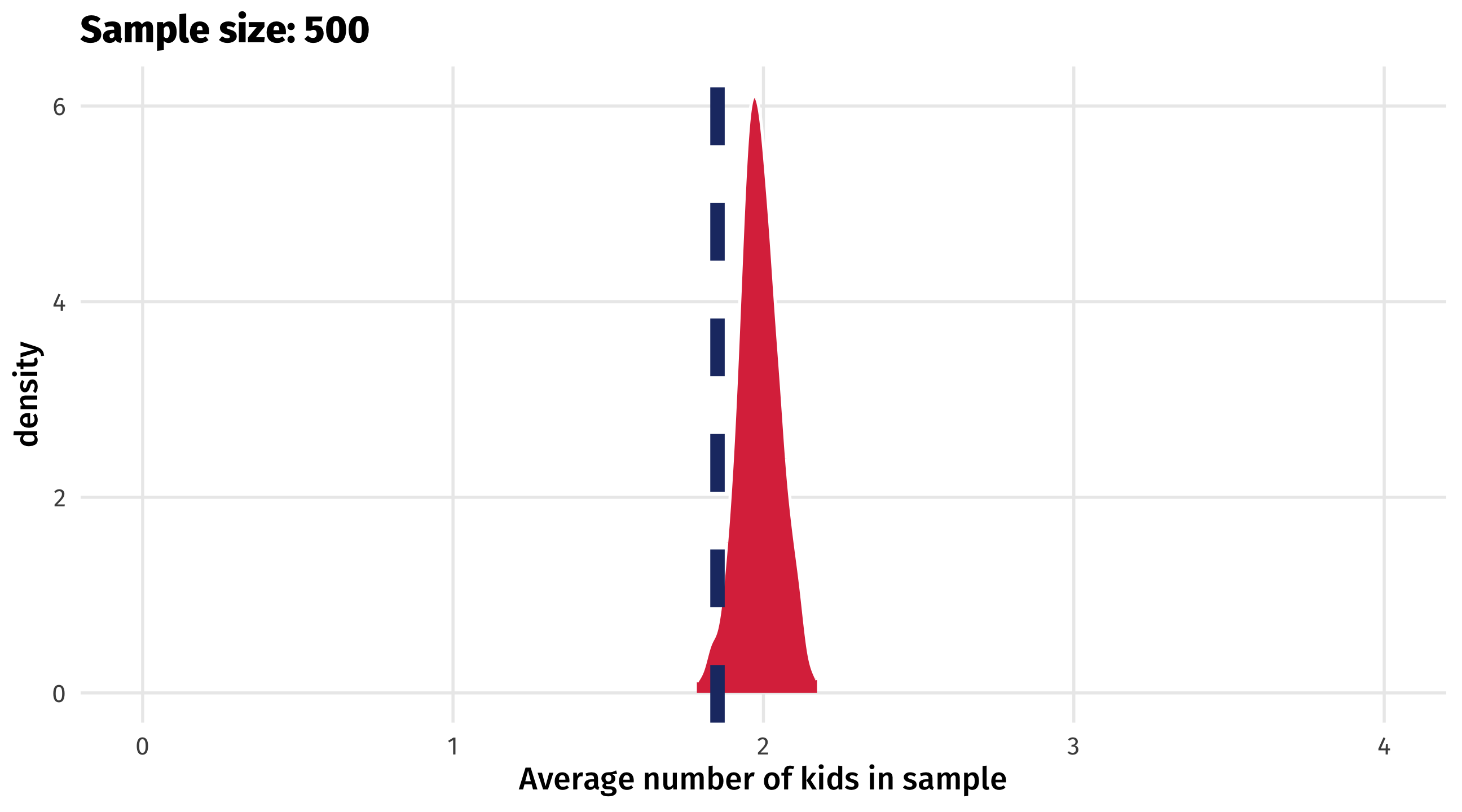
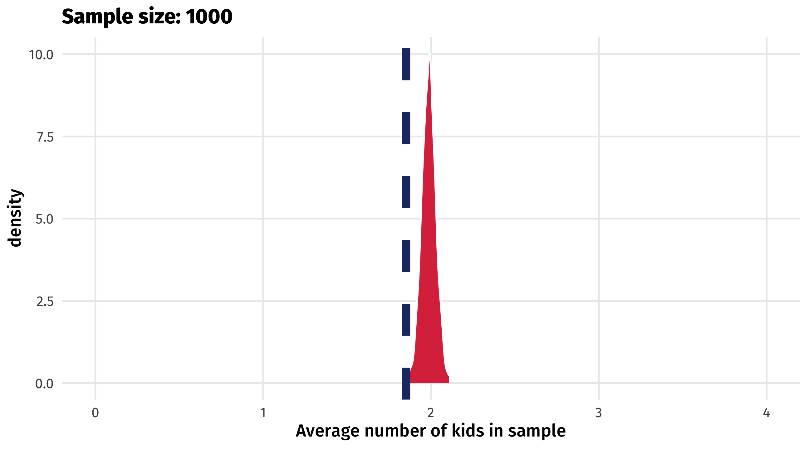
With a small sample, estimates can vary a lot:

Law of large numbers

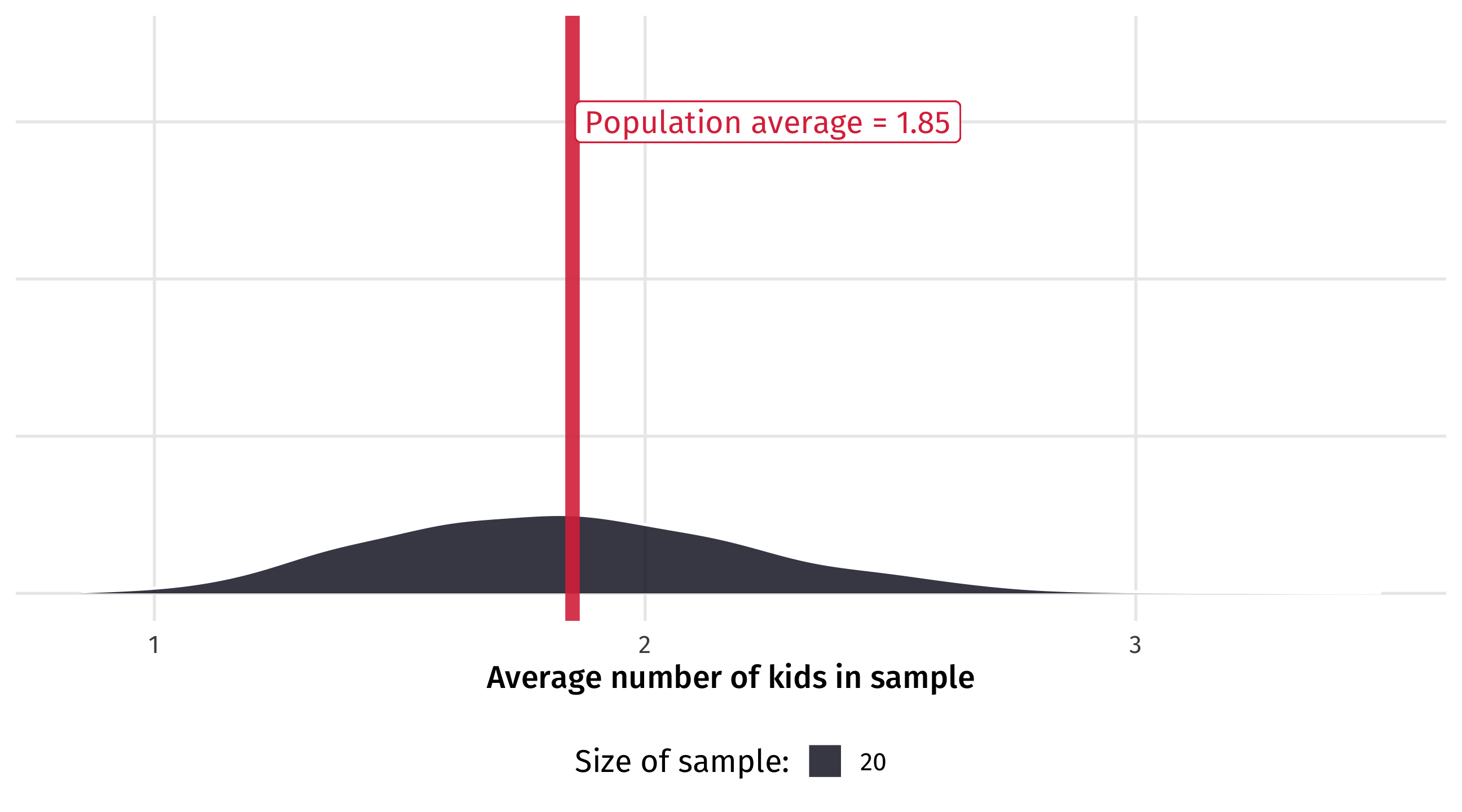
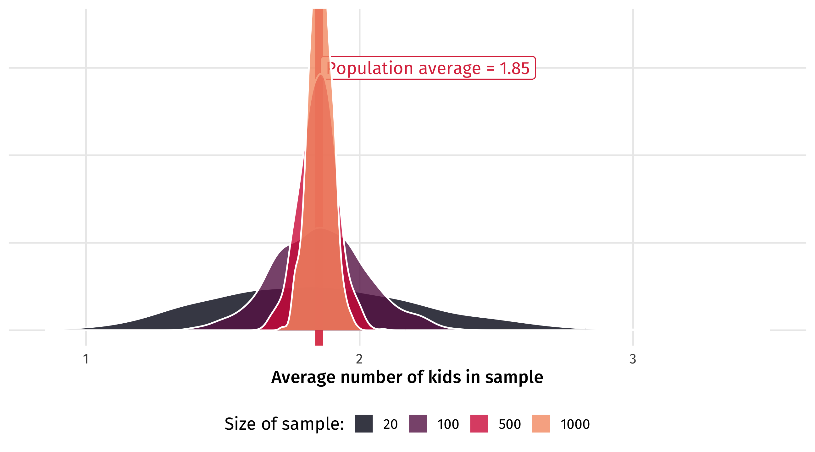
As the sample size (N) increases, estimates begin to converge:

Law of large numbers

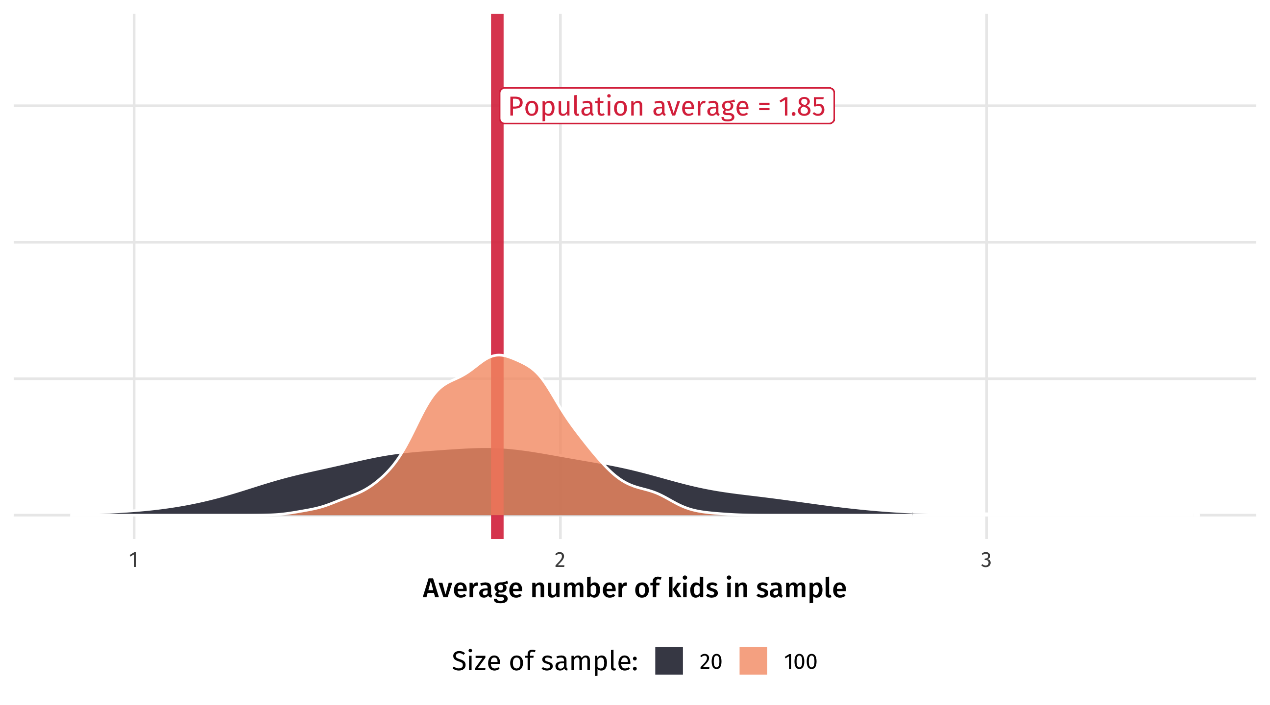
They become more concentrated around the population average…

Law of large numbers

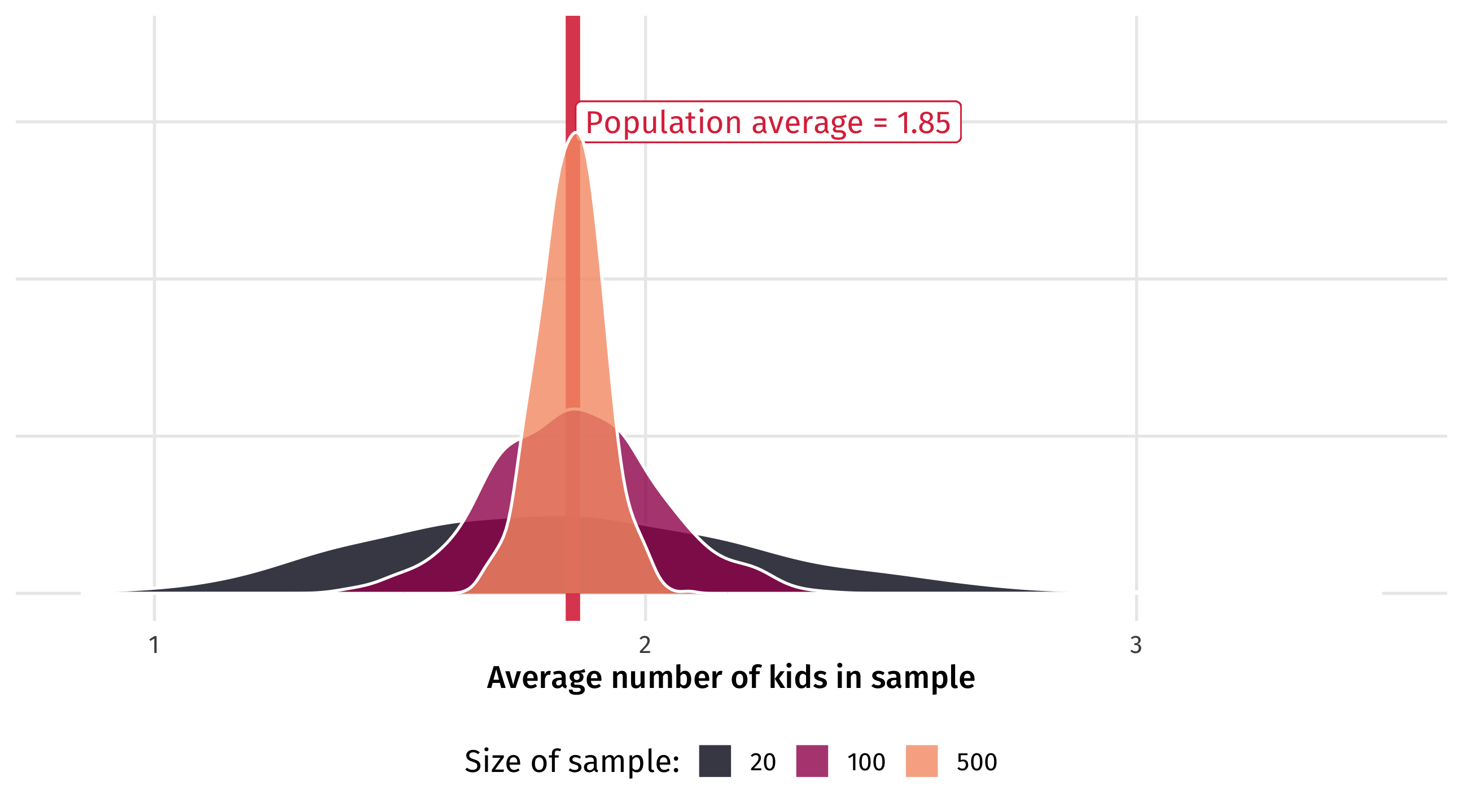
And eventually it becomes very unlikely the sample estimate is way off

This works for regression estimates, too

Regression estimates also become more precise as sample size increases:

What’s going on?

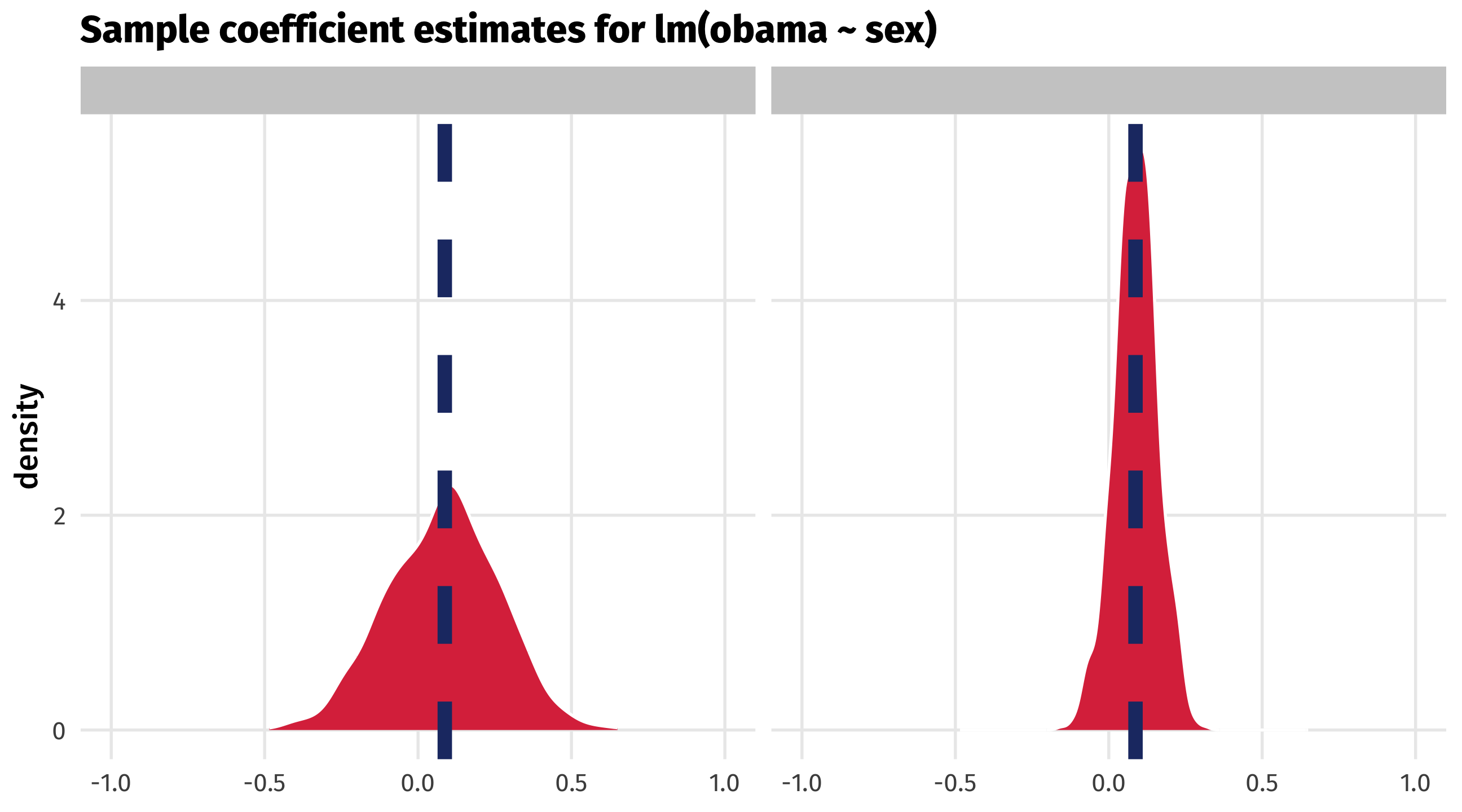
The larger our sample, the less likely it is that our estimate (average number of kids, the effect of sex on vote choice, etc.) is way off

This is because as sample size increases, sample estimates tend to converge on the population parameter

Next time = we’ll see how to quantify uncertainty based on this tendency

Intuitive = the more data we have, the less uncertain we should feel

But this only works if we have a good sample

Good and bad samples

There are good and bad samples in the world

Good sample representative of the population and unbiased

Bad sample the opposite of a good sample

What does this mean?

When sampling goes wrong

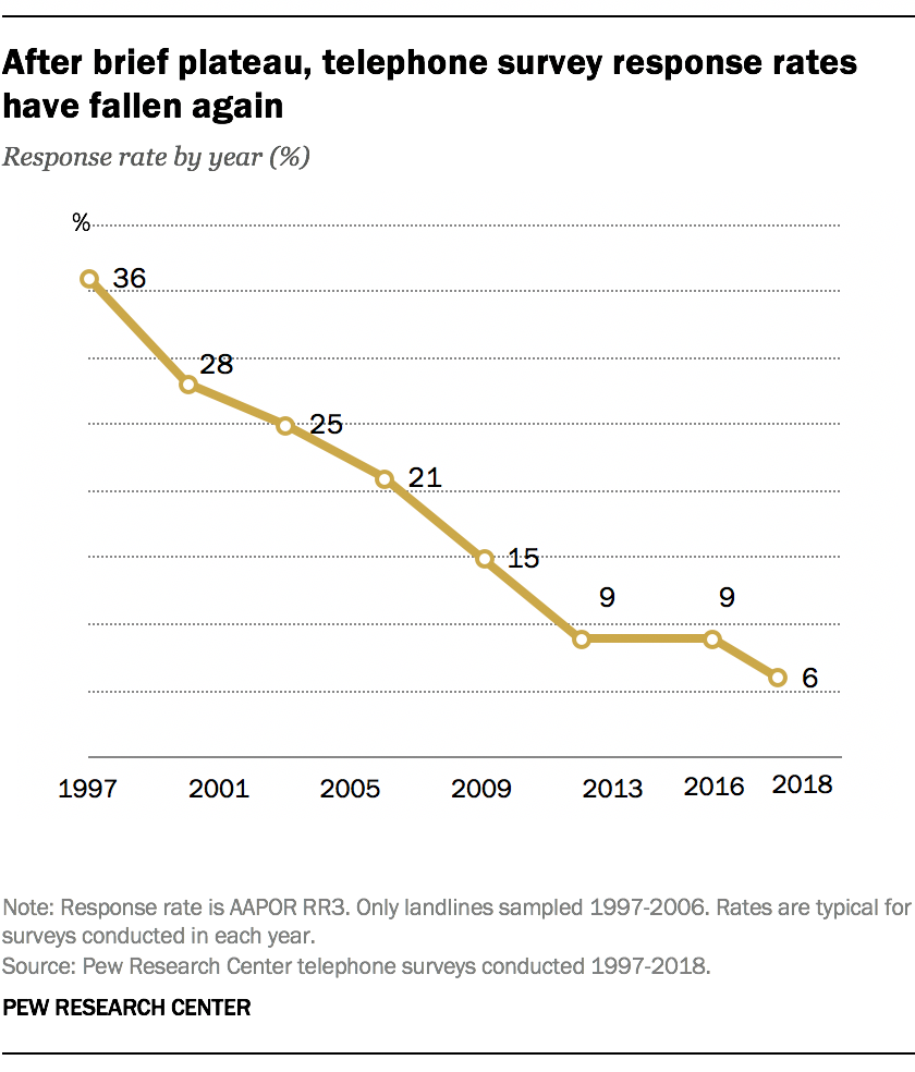
Imagine that in our quest to find out how many kids the average American has, we do telephone surveys

Younger people are less likely to have a landline than older people, so few young people make it onto our survey

what happens to our estimate?

When sampling goes wrong

We can simulate this by again pretending gss_sm is the whole of the US

Let’s imagine the extreme scenario where no one under 25 makes it into the survey:

gss_sm %>% 
  filter(age >= 25) %>%
  rep_sample_n(size = 10, reps = 1000) %>% 
  summarise(avg_kids = mean(childs, na.rm = TRUE))

I’ve filtered out all people in gss_sm under 25 so they cannot be sampled

When sampling goes wrong

As sample size increases, variability of estimates will still decrease

When sampling goes wrong

But estimates will be biased, regardless of sample size

What’s going on?

The sample is not representative of the population (the young people are missing)

This biases our estimate of the population parameter

Randomness is key = everyone needs a similar chance of ending up in the sample

When young people don’t have land-lines, not everyone has a similar chance of ending up in the sample

A big problem!

🚨 Your turn: bias the polls 🚨

Imagine you are an evil pollster:

Think about who you would have to exclude from the data to create estimates that benefit the pro-choice and pro-life side of the abortion debate.
Explain how you think this change would effect the estimate variability as the sample size increases or decreases.

# So… Where are we at?

The problem

We know our analysis is based on samples, and different samples give different answers:

Sample	Avg. num of kids in sample
1	1.3
2	2.2
3	1.5
4	1.0
5	1.5
6	0.7
7	1.8
8	1.8

The way out

Turns out that if our samples are representative of the population, then estimates from large samples will tend to be pretty damn close
So if sample is good ✅ and “big” ✅ then most of the time we’ll be OK ✅

But this is weird

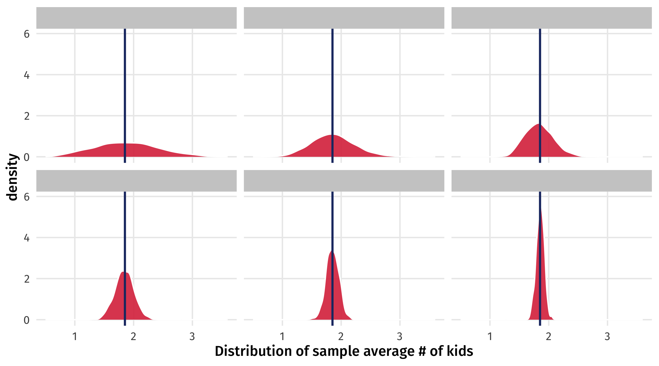
We’ve shown that if we take many (large) random samples, most of the averages of those samples will be close to population parameter

But in real life we only ever have one sample (e.g., one poll)

How do we get a sense for uncertainty from our one sample?

Two approaches

❌ ~~Statistical theory~~

Make assumptions about distribution of samples from population
Design test based on those assumptions (t-test, z-test, etc.)

✅ Simulation

Simulate different samples that look like ours
Use distribution of simulated samples to quantify uncertainty

In some cases, both get you to the same answer, in others, only one works

Simulation

We want a sense for how uncertain we should feel on estimates drawn from our sample

Our sample is gss_sm, and we have 2,867 observations

gss_sm
year	id	ballot	age	childs	sibs	degree	race
2016	624	3	57	2	11	High School	Black
2016	908	2	47	0	4	High School	White
2016	2817	2	53	3	2	Bachelor	White
2016	2249	2	62	4	3	High School	Black
2016	2071	2	28	0	5	Junior College	White

How confident are we in the estimate we get from this sample, given its size?

How to simulate

If we take lots of samples of size 20 \(\rightarrow\) uncertainty in a sample of 20

gss_sm %>%
  rep_sample_n(size = 20, reps = 1000)

How to simulate

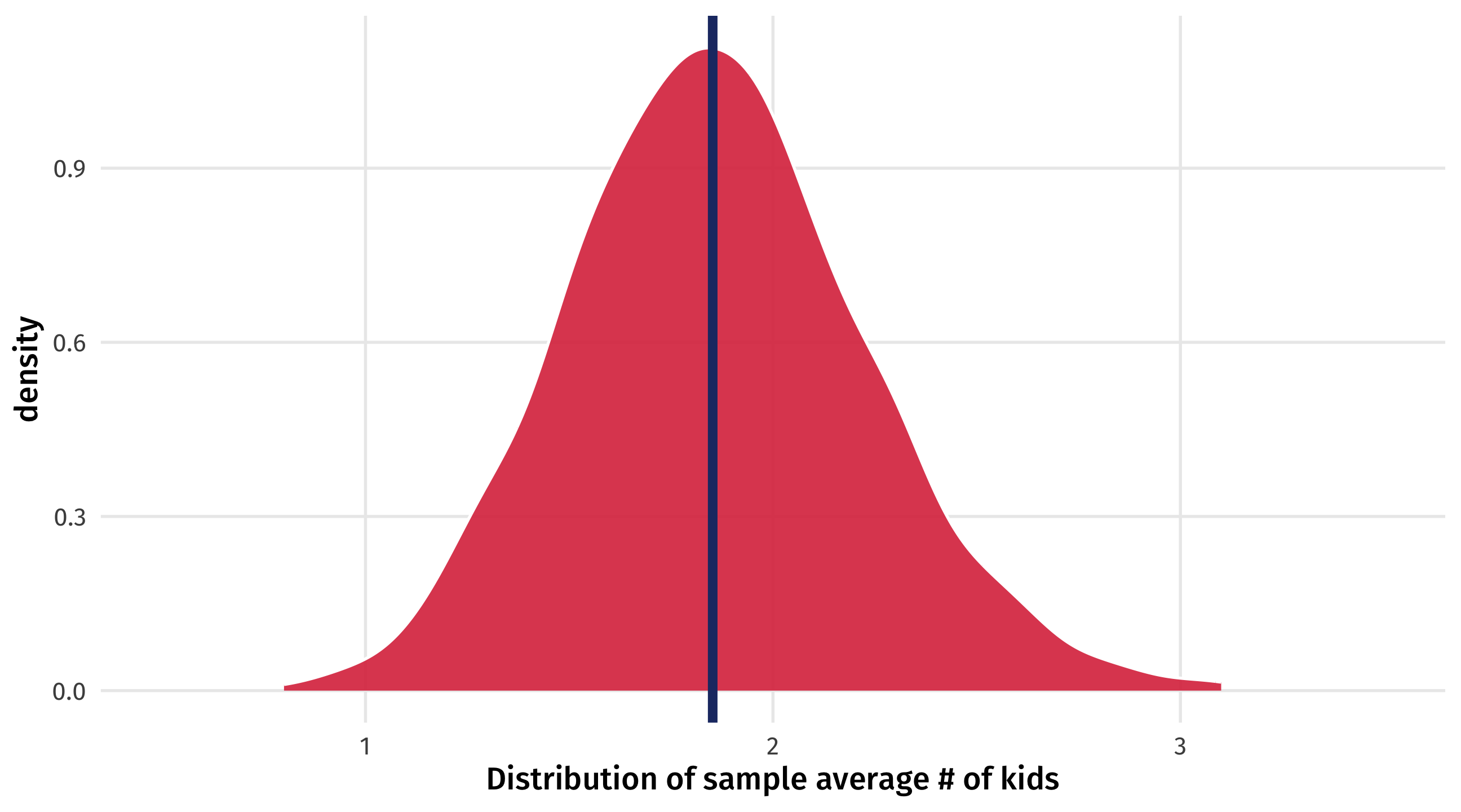
If we take lots of samples of size 100 \(\rightarrow\) uncertainty in a sample of 100

gss_sm %>%
  rep_sample_n(size = 100, reps = 1000)

How to simulate

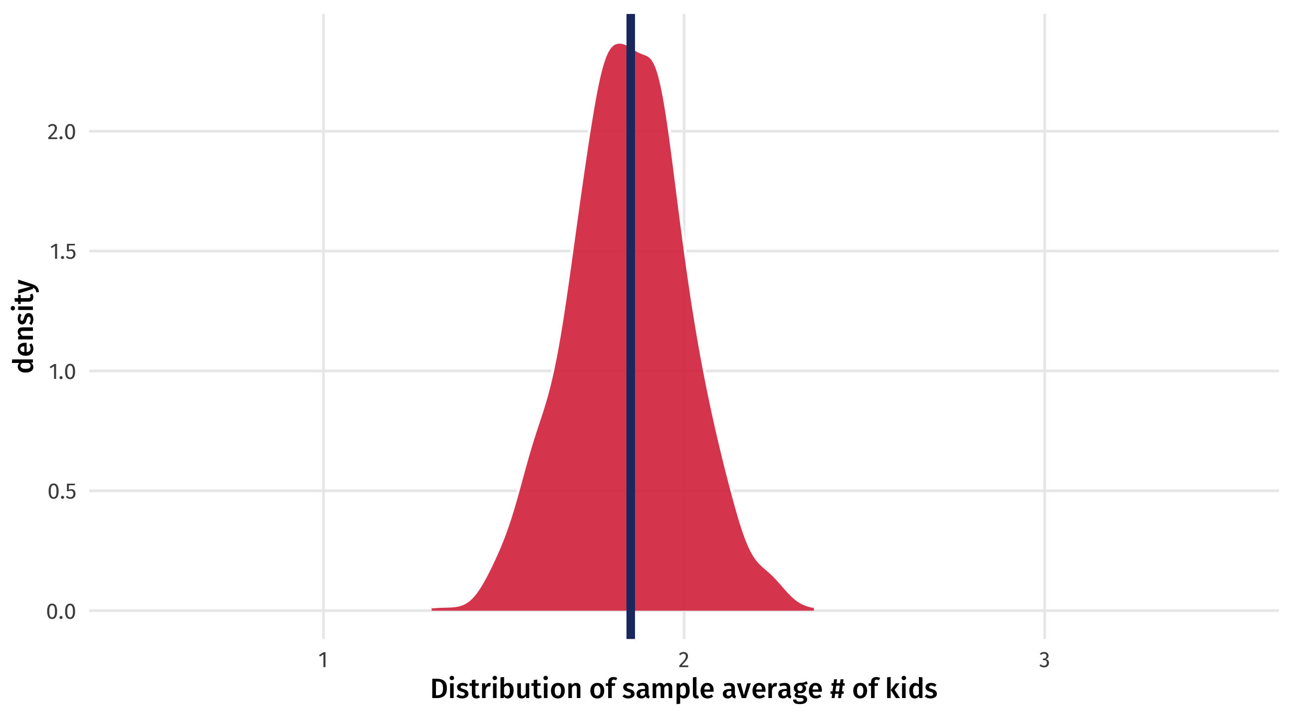
So to see how uncertain we should feel about gss_sm, we should take many samples that are the same size as gss_sm

gss_sm %>% 
  rep_sample_n(size = 2867, reps = 1000)

Note

nrow(DATA) tells you how many observations in data object

Problem

If we have a dataset of 2,867 observations and ask R to randomly pick 2,867 observations, we’ll just get a bunch of copies of the original dataset

gss_sm %>% 
  rep_sample_n(size = nrow(gss_sm), reps = 1000)

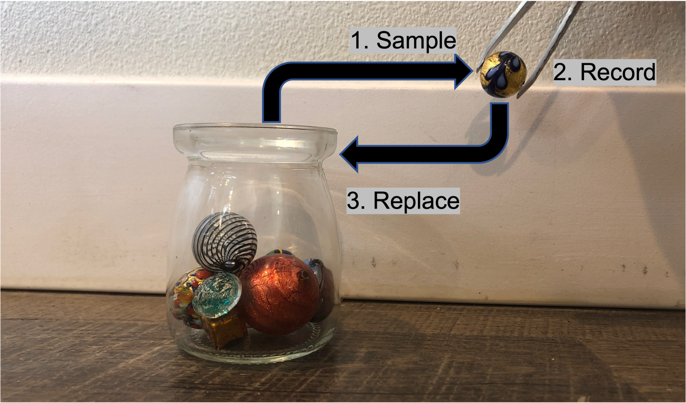
Solution: sample with replacement \(\rightarrow\) once we draw an observation it goes back into the dataset, ad can be sampled again

gss_sm %>% 
  rep_sample_n(size = nrow(gss_sm), reps = 1000, replace = TRUE)

Sampling with replacement

Sampling with and without replacement

If we were sampling 4 of these delicious fruits:

fruits = c("Mango", "Pineapple", "Banana", "Blackberry")
fruits

[1] "Mango"      "Pineapple"  "Banana"     "Blackberry"

It would look like this, with and without replacement:

Sample, no replace	Mango	Banana	Pineapple	Blackberry
Sample, replace	Pineapple	Pineapple	Banana	Blackberry

Bootstrapping

Generating many, same-sized samples with replacement is called bootstrapping
Replacement lets us generate samples that randomly differ from ours
Use the distribution of bootstrapped samples to quantify uncertainty

Only one sample? Pull yourself up by your bootstraps!

Back to the kids

How uncertain should we be of our estimate of the avg. number of kids in the US, Given that it’s based on our one sample, gss_sm? We can bootstrap:

boot_kids = gss_sm %>% 
  rep_sample_n(size = nrow(gss_sm), reps = 1000, replace = TRUE) %>% 
  summarise(avg_kids = mean(childs, na.rm = TRUE))
boot_kids

# A tibble: 1,000 × 2
   replicate avg_kids
       <int>    <dbl>
 1         1     1.88
 2         2     1.85
 3         3     1.88
 4         4     1.87
 5         5     1.88
 6         6     1.87
 7         7     1.83
 8         8     1.84
 9         9     1.82
10        10     1.77
# ℹ 990 more rows

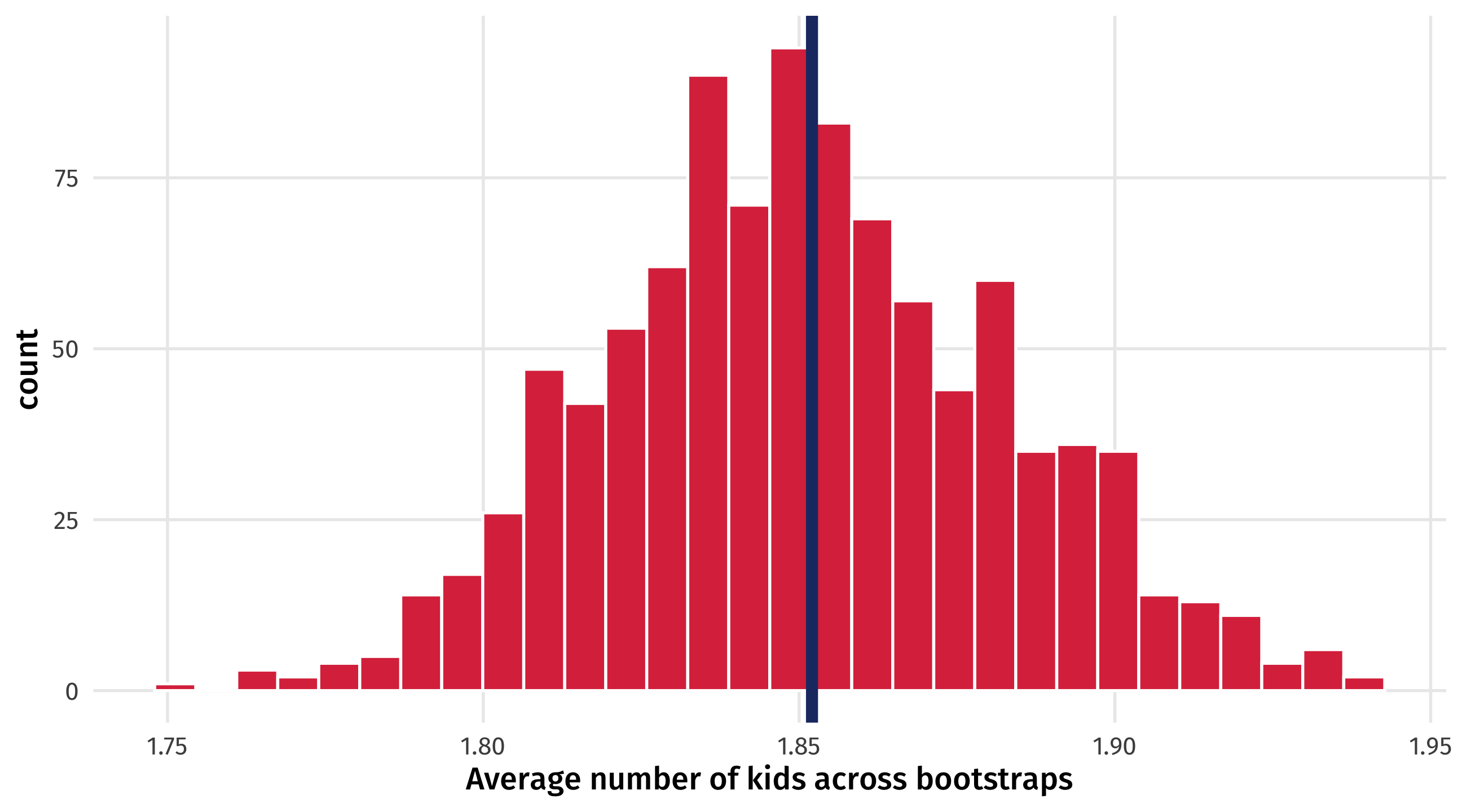
The distribution of bootstrapped estimates

Our estimate and how much simulated estimates might vary across bootstrapped samples that look like ours

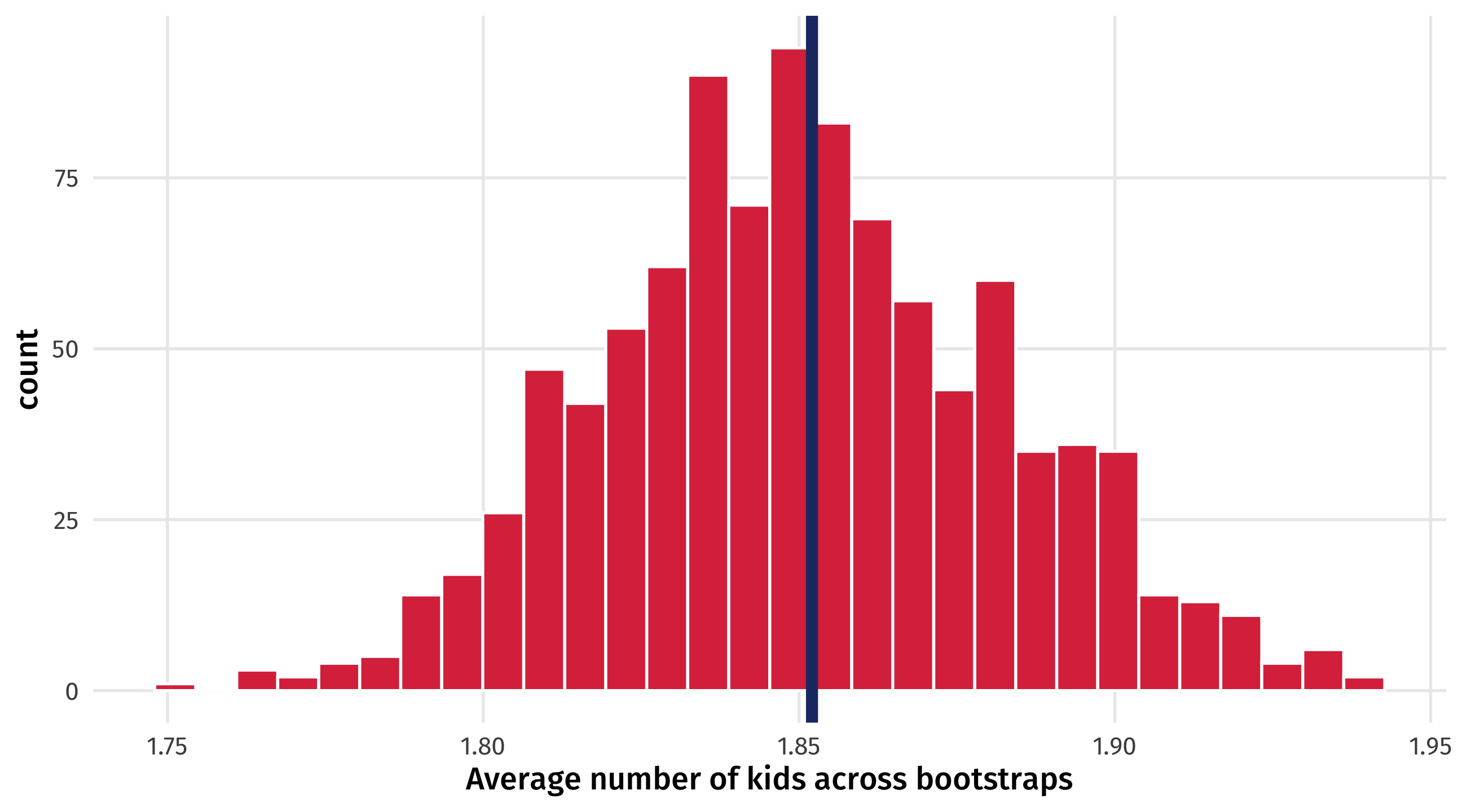
The red is the distribution of bootstrapped sample estimates \(\rightarrow\) the sampling distribution

# Quantifying uncertainty

How to quantify uncertainty?

The red histogram is nice, but how can we communicate uncertainty in our estimates in a pithy, more comparable way?

Three approaches:

The standard error
The confidence interval
Statistical significance

The standard error

One way to quantify uncertainty would be to measure how “wide” the distribution of bootstrapped sample estimates is

As we learned so long ago, one way to measure the “spread” of a distribution (i.e., how much a variable varies), is with the standard deviation

The standard deviation of the sampling distribution is called the standard error, or the margin of error

boot_kids %>% 
  summarise(mean = mean(avg_kids), 
            standard_error = sd(avg_kids))

# A tibble: 1 × 2
   mean standard_error
  <dbl>          <dbl>
1  1.85         0.0319

Best guess on how many kids the average American has? About 1.85 kids, +/- 2 standard errors

Standard error

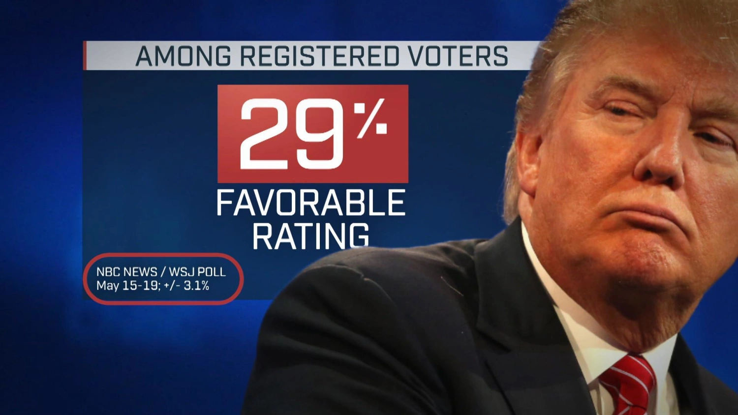
This is what you see in the news – that +/- polling/margin of error

Varying uncertainty

As our sample size increases, the standard error decreases

Sample size	Average (truth = 10)	Standard error
10.00	9.12	0.74
64.44	10.06	0.28
118.89	10.11	0.19
173.33	10.07	0.16
227.78	9.89	0.13
282.22	9.94	0.12
336.67	10.00	0.11
391.11	10.08	0.10
445.56	9.99	0.09
500.00	9.92	0.09

The confidence interval

Another way to quantify uncertainty is to look where most estimates fall

this is the confidence interval: our “best guess” of what we’re trying to estimate

How big to make the interval?

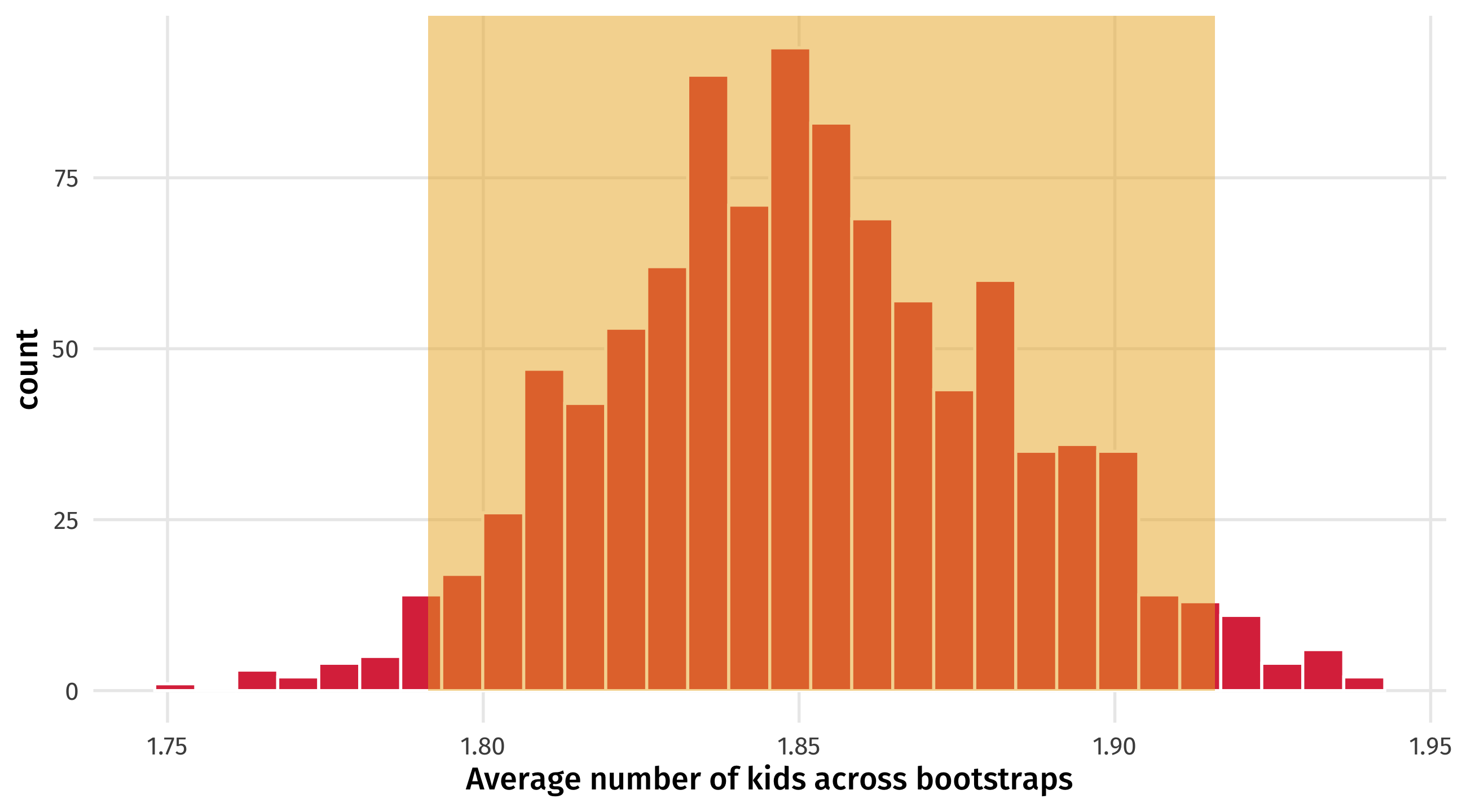
You could report (for example) where the middle 50% of bootstraps fall, or (for example) where the middle 95% of bootstraps fall, but there are tradeoffs!

The tradeoff

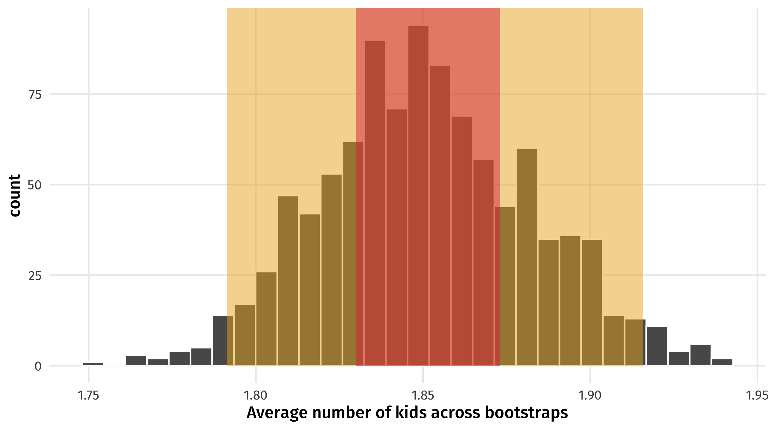
You are 50% “confident” that avg. number of kids could vary between 1.83 and 1.87. Narrower range! But low confidence!
You are 95% “confident” that avg. number of kids could vary between 1.79 and 1.92. Higher range! But higher confidence!

How big to make the interval?

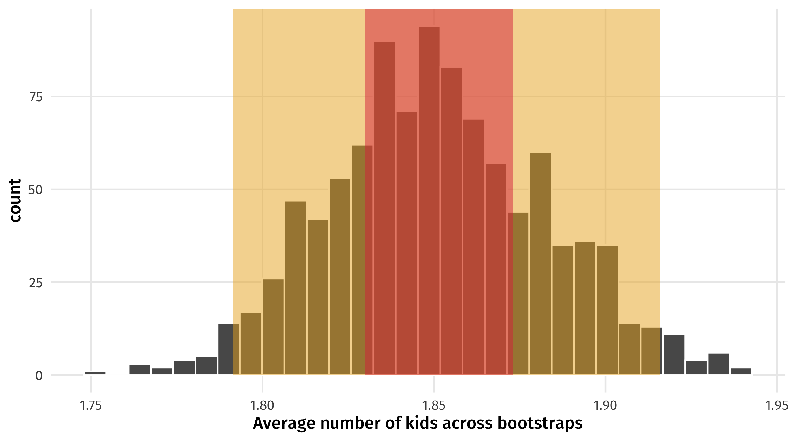
Convention is to look at the middle 95% of the distribution

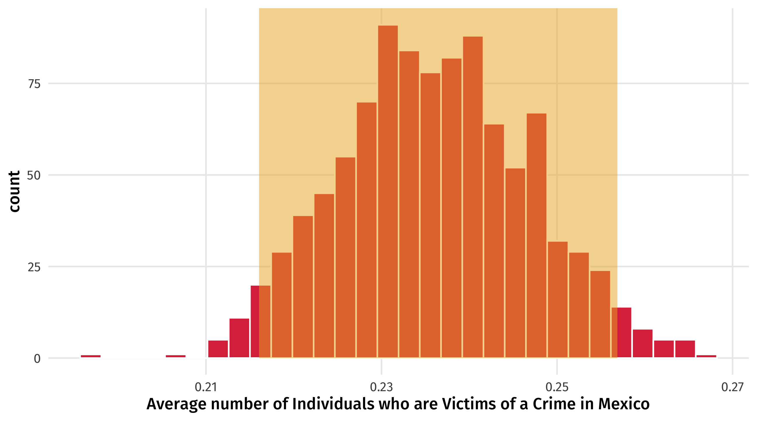
Where do the middle 95% of the bootstrap estimates fall?

We can use the quantile() function to get here

boot_kids %>% 
  summarise(low = quantile(avg_kids, .025), # middle 95% means lower bound is .025
            mean = mean(avg_kids), 
            high = quantile(avg_kids, .975)) # middle 95% means upper bound is .975

# A tibble: 1 × 3
    low  mean  high
  <dbl> <dbl> <dbl>
1  1.79  1.85  1.92

The 95% confidence confidence interval for the average number of kids in the US is: (1.80, 1.91)

Mirrors of one another

The standard error and confidence interval are actually telling you the same thing

A 95% confidence interval is roughly equal to the Estimate +/- 1.96 \(\times\) standard error

boot_kids %>% 
  summarise(low = quantile(avg_kids, .025),
            mean = mean(avg_kids), 
            high = quantile(avg_kids, .975))

# A tibble: 1 × 3
    low  mean  high
  <dbl> <dbl> <dbl>
1  1.79  1.85  1.92

boot_kids %>% 
  summarise(mean = mean(avg_kids), standard_error = sd(avg_kids)) %>% 
  mutate(low = mean - 1.96 * standard_error, 
         high = mean + 1.96 * standard_error) %>% 
  select(low, mean, high)

# A tibble: 1 × 3
    low  mean  high
  <dbl> <dbl> <dbl>
1  1.79  1.85  1.91

🚨 Your turn: polling crime victimization 🚨

Use the crime data, and:

Pick a pais of your choosing. What proportion of respondents have been a victim of a crime in the last 12 months (vic1ext) in that country?
OK, but how certain are you of that? Generate 1,000 bootstraps.
Calculate the standard error and the 95% confidence interval of your best guess. Convince yourself the two can be made equivalent.

Note

Use distinct() to find a country (pias), use filter() to use that region
boot_data = data |>

rep_sample_n(size = nrow(data), reps = 1000, replace = TRUE) |>

summarise(avg = mean(variable, na.rm = TRUE),

standard_error = sd(variable, na.rm = TRUE))|>

mutate(low = avg - 1.96 * standard_error,

high = avg + 1.96 * standard_error)

🚨 Example: Polling Crime Victimization 🚨

library(juanr)

data <- crime |>
  filter(pais == "Mexico")

boot_data = data |> 
  rep_sample_n(size = nrow(data), reps = 1000, replace = TRUE) |> 
  summarise(avg = mean(vic1ext, na.rm = TRUE),
            standard_error = sd(vic1ext, na.rm = TRUE)) |>
  mutate(low = avg - 1.96 * standard_error, 
         high = avg + 1.96 * standard_error)