In the following coding examples, you will see three important functions, a pipe, select(), and filter().
Pipes (%>% or |>)
First, a pipe is written as a %>% or |>. Pipes are a powerful tool that help us clearly express a sequence of functions. Pipes tell R that you want to use a designated set for a chain of functions that build off of each other. A way to think about this is in math terms.
\[ F(G(H(X))), X=Data\]
In this series of functions, the first step is you solve \(H(X)\), then using that solution you solve \(G()\), then after you solve \(F()\). The final output is the solution of those chain of events with the information of \(X\). This is how pipes work! Pipes use a set of information, typically a data frame, and then apply it to a series of functions that build off each other.
Filter() and Select()
In the following example, I use the select() and filter() to simplify the data. The select() allows me to select certain variables from the data and eliminate the rest. filter() does something similar but instead of variables, it allows me to simplify the data based on values based on a set of programmed logical operators. In my first example, I select for the circuit, year, constructor, surname of the driver, and the number of points awarded during that race. I use the unique() to remove duplicates, and then I filter for the race information for the constructor McLaren during the 2023 season.
library(tidyverse)
── Attaching core tidyverse packages ──────────────────────── tidyverse 2.0.0 ──
✔ dplyr     1.2.1     ✔ readr     2.2.0
✔ forcats   1.0.1     ✔ stringr   1.6.0
✔ ggplot2   4.0.3     ✔ tibble    3.3.1
✔ lubridate 1.9.5     ✔ tidyr     1.3.2
✔ purrr     1.2.2
── Conflicts ────────────────────────────────────────── tidyverse_conflicts() ──
✖ dplyr::filter() masks stats::filter()
✖ dplyr::lag()    masks stats::lag()
ℹ Use the conflicted package (<http://conflicted.r-lib.org/>) to force all conflicts to become errors
# A tibble: 40 × 5
   circuit                         year constructor surname points
   <chr>                          <dbl> <chr>       <chr>    <dbl>
 1 Bahrain International Circuit   2023 McLaren     Norris       0
 2 Jeddah Corniche Circuit         2023 McLaren     Norris       0
 3 Jeddah Corniche Circuit         2023 McLaren     Piastri      0
 4 Albert Park Grand Prix Circuit  2023 McLaren     Norris       8
 5 Albert Park Grand Prix Circuit  2023 McLaren     Piastri      4
 6 Baku City Circuit               2023 McLaren     Norris       2
 7 Baku City Circuit               2023 McLaren     Piastri      0
 8 Miami International Autodrome   2023 McLaren     Norris       0
 9 Miami International Autodrome   2023 McLaren     Piastri      0
10 Circuit de Monaco               2023 McLaren     Norris       2
# ℹ 30 more rows
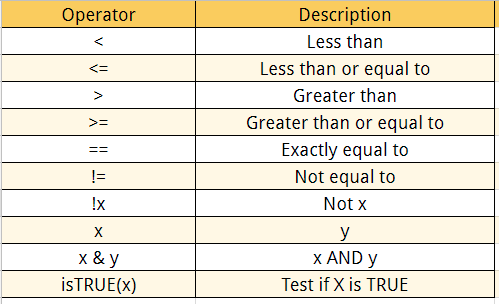
What if we wanted two different constructors? Then we want to use the logical operator for | and also differentiate it from the next instruction for filter by using a , or (). In the example below, I filter for the race information for the constructor Mercedes and Red Bull during the 2021 season.
# A tibble: 80 × 5
   circuit                             year constructor surname  points
   <chr>                              <dbl> <chr>       <chr>     <dbl>
 1 Losail International Circuit        2021 Mercedes    Hamilton     25
 2 Losail International Circuit        2021 Mercedes    Bottas        0
 3 Bahrain International Circuit       2021 Mercedes    Hamilton     25
 4 Bahrain International Circuit       2021 Mercedes    Bottas       16
 5 Autodromo Enzo e Dino Ferrari       2021 Mercedes    Hamilton     19
 6 Autodromo Enzo e Dino Ferrari       2021 Mercedes    Bottas        0
 7 Autódromo Internacional do Algarve  2021 Mercedes    Hamilton     25
 8 Autódromo Internacional do Algarve  2021 Mercedes    Bottas       16
 9 Circuit de Barcelona-Catalunya      2021 Mercedes    Hamilton     25
10 Circuit de Barcelona-Catalunya      2021 Mercedes    Bottas       15
# ℹ 70 more rows
However, if we wanted to use the modified data, we could not because it is not saved. If we want to use this data we need to save it as a new object!
# A tibble: 80 × 5
   circuit                             year constructor surname  points
   <chr>                              <dbl> <chr>       <chr>     <dbl>
 1 Losail International Circuit        2021 Mercedes    Hamilton     25
 2 Losail International Circuit        2021 Mercedes    Bottas        0
 3 Bahrain International Circuit       2021 Mercedes    Hamilton     25
 4 Bahrain International Circuit       2021 Mercedes    Bottas       16
 5 Autodromo Enzo e Dino Ferrari       2021 Mercedes    Hamilton     19
 6 Autodromo Enzo e Dino Ferrari       2021 Mercedes    Bottas        0
 7 Autódromo Internacional do Algarve  2021 Mercedes    Hamilton     25
 8 Autódromo Internacional do Algarve  2021 Mercedes    Bottas       16
 9 Circuit de Barcelona-Catalunya      2021 Mercedes    Hamilton     25
10 Circuit de Barcelona-Catalunya      2021 Mercedes    Bottas       15
# ℹ 70 more rows
Now, we can use this information!
Logical Operators
Base R Descriptive Stats
First, let’s find the minimum speed recorded and the maximum speed recorded during the fastest laps for each race. Since fastest lap time is a character we need to change it from a character to a numeric value, and let’s remove any NAs.
library(RandomData)dat <- race_stats# change NA to 0s and to numericdat$fastestLapSpeed <-as.numeric(ifelse(dat$fastestLapSpeed >=0, dat$fastestLapSpeed, 0) )
Min and Max
min(dat$fastestLapSpeed)
[1] 0
max(dat$fastestLapSpeed)
[1] 255.014
range(dat$fastestLapSpeed)
[1] 0.000 255.014
Mean
The mean is the average value of all the numbers in a set.
mean(dat$fastestLapSpeed)
[1] 201.4552
Median
The median is the middle value in a set of numbers when they are ordered from least to greatest.
median(dat$fastestLapSpeed)
[1] 203.003
First and Third Quartiles
The first quartile range is the value under which 25 percent of the data points are found when they are arranged in increasing order, and the third quartile range is where 75 percent of the data points are found when they are arranged in increasing order
quantile(dat$fastestLapSpeed, 0.25)
    25%
191.142
quantile(dat$fastestLapSpeed, 0.75)
    75%
214.339
IQR
The IQR is the difference between the first and third quartile.
IQR(dat$fastestLapSpeed)
[1] 23.197
Standard Deviation and Variance
Variance is the average squared difference between data points in a set, which measures how much the values in a set vary from each other, while Standard Deviation is the measure of how far the values in a set are from the mean
sd(dat$fastestLapSpeed)
[1] 23.22281
var(dat$fastestLapSpeed)
[1] 539.2991
Creating New Variables
We can also add to our data sets! If we want to make a new variable, we can use the mutate(), which uses existing data to create new variables. The correct format of the function is the following, first is the new variable name and then an equal sign =, followed by how the new variable will be formed and what existing variables are used to make it.
# A tibble: 40 × 5
   circuit                         year constructor surname avg_laptime
   <chr>                          <dbl> <chr>       <chr>         <dbl>
 1 Bahrain International Circuit   2023 McLaren     Norris      646286.
 2 Jeddah Corniche Circuit         2023 McLaren     Norris      710915.
 3 Jeddah Corniche Circuit         2023 McLaren     Piastri     710915.
 4 Albert Park Grand Prix Circuit  2023 McLaren     Norris      612858.
 5 Albert Park Grand Prix Circuit  2023 McLaren     Piastri     612858.
 6 Baku City Circuit               2023 McLaren     Norris      696975.
 7 Baku City Circuit               2023 McLaren     Piastri     696975.
 8 Miami International Autodrome   2023 McLaren     Norris      623609.
 9 Miami International Autodrome   2023 McLaren     Piastri     634745.
10 Circuit de Monaco               2023 McLaren     Norris      461633.
# ℹ 30 more rows
If we wanted to make a new character variable we would use the case_when() in the mutate() function. In this example, I make a new variable based on the final position of the race for the two McLaren drivers, Piastri and Norris, in the 2023 season. I use the existing variables the circuit and surname to make this new variable.
McLarenStandings_2023 <- race_stats |>select(circuit, year, constructor, surname) |># remove duplicatesunique() |>filter(constructor =="McLaren"& year ==2023) |>mutate(final_position =case_when(#PIASTRI circuit =="Bahrain International Circuit"& surname =="Piastri"~"DNF", circuit =="Jeddah Corniche Circuit"& surname =="Piastri"~"15", circuit =="Albert Park Grand Prix Circuit"& surname =="Piastri"~"8", circuit =="Baku City Circuit"& surname =="Piastri"~"11", circuit =="Miami International Autodrome"& surname =="Piastri"~"19", circuit =="Circuit de Monaco"& surname =="Piastri"~"10", circuit =="Circuit de Barcelona-Catalunya"& surname =="Piastri"~"13", circuit =="Circuit Gilles Villeneuve"& surname =="Piastri"~"11", circuit =="Red Bull Ring"& surname =="Piastri"~"16", circuit =="Silverstone Circuit"& surname =="Piastri"~"4", circuit =="Hungaroring"& surname =="Piastri"~"5", circuit =="Circuit de Spa-Francorchamps"& surname =="Piastri"~"DNF", circuit =="Circuit Park Zandvoort"& surname =="Piastri"~"9", circuit =="Autodromo Nazionale di Monza"& surname =="Piastri"~"12", circuit =="Marina Bay Street Circuit"& surname =="Piastri"~"7", circuit =="Suzuka Circuit"& surname =="Piastri"~"3", circuit =="Losail International Circuit"& surname =="Piastri"~"2", circuit =="Circuit of the Americas"& surname =="Piastri"~"DNF", circuit =="Autódromo Hermanos Rodríguez"& surname =="Piastri"~"8", circuit =="Autódromo José Carlos Pace"~"14", circuit =="Las Vegas Strip Street Circuit"& surname =="Piastri"~"10", circuit =="Yas Marina Circuit"& surname =="Piastri"~"6",# NORRIS circuit =="Bahrain International Circuit"& surname =="Norris"~"17", circuit =="Jeddah Corniche Circuit"& surname =="Norris"~"17", circuit =="Albert Park Grand Prix Circuit"& surname =="Norris"~"6", circuit =="Baku City Circuit"& surname =="Norris"~"9", circuit =="Miami International Autodrome"& surname =="Norris"~"17", circuit =="Circuit de Monaco"& surname =="Norris"~"9", circuit =="Circuit de Barcelona-Catalunya"& surname =="Norris"~"17", circuit =="Circuit Gilles Villeneuve"& surname =="Norris"~"13", circuit =="Red Bull Ring"& surname =="Norris"~"4", circuit =="Silverstone Circuit"& surname =="Norris"~"2", circuit =="Hungaroring"& surname =="Norris"~"2", circuit =="Circuit de Spa-Francorchamps"& surname =="Norris"~"7", circuit =="Circuit Park Zandvoort"& surname =="Norris"~"9", circuit =="Autodromo Nazionale di Monza"& surname =="Norris"~"8", circuit =="Marina Bay Street Circuit"& surname =="Norris"~"2", circuit =="Suzuka Circuit"& surname =="Norris"~"2", circuit =="Losail International Circuit"& surname =="Norris"~"3", circuit =="Circuit of the Americas"& surname =="Norris"~"3", circuit =="Autódromo Hermanos Rodríguez"& surname =="Norris"~"5", circuit =="Autódromo José Carlos Pace"~"2", circuit =="Las Vegas Strip Street Circuit"& surname =="Norris"~"DNF", circuit =="Yas Marina Circuit"& surname =="Norris"~"5" ) ) print(McLarenStandings_2023)
# A tibble: 40 × 5
   circuit                         year constructor surname final_position
   <chr>                          <dbl> <chr>       <chr>   <chr>
 1 Bahrain International Circuit   2023 McLaren     Norris  17
 2 Jeddah Corniche Circuit         2023 McLaren     Norris  17
 3 Jeddah Corniche Circuit         2023 McLaren     Piastri 15
 4 Albert Park Grand Prix Circuit  2023 McLaren     Norris  6
 5 Albert Park Grand Prix Circuit  2023 McLaren     Piastri 8
 6 Baku City Circuit               2023 McLaren     Norris  9
 7 Baku City Circuit               2023 McLaren     Piastri 11
 8 Miami International Autodrome   2023 McLaren     Norris  17
 9 Miami International Autodrome   2023 McLaren     Piastri 19
10 Circuit de Monaco               2023 McLaren     Norris  9
# ℹ 30 more rows
Descriptive Statistics Using Tidyverse
Now that we know some basic ways to manipulate the data frame, let’s look at different ways to do basic descriptive statistics! In this section we will be using the function, summarize(). This function is similar to the mutate function, except instead of adding a variable, it makes a new data frame based on existing variables. You will also see the function group_by(). This function allows us to organize the data by telling it to group things by a variable(s). Essentially, the functions splits things into groups.
For this example we are going to find the total points for each team in the 2023 season!
# A tibble: 10 × 2
   constructor    total_points
   <chr>                 <dbl>
 1 Alfa Romeo               16
 2 AlphaTauri               22
 3 Alpine F1 Team          110
 4 Aston Martin            266
 5 Ferrari                 363
 6 Haas F1 Team              9
 7 McLaren                 266
 8 Mercedes                374
 9 Red Bull                790
10 Williams                 26
# A tibble: 10 × 2
   constructor    total_points
   <chr>                 <dbl>
 1 Red Bull                790
 2 Mercedes                374
 3 Ferrari                 363
 4 Aston Martin            266
 5 McLaren                 266
 6 Alpine F1 Team          110
 7 Williams                 26
 8 AlphaTauri               22
 9 Alfa Romeo               16
10 Haas F1 Team              9
What if we wanted to know the percentage of points each driver contributed to the teams total?
TeamStandings_2023 <- race_stats |>select(circuit, year, constructor, surname, points) |># remove duplicatesunique() |>filter(year==2023) |>group_by(constructor) |>mutate(total_points =sum(points, na.rm =TRUE)) |>ungroup() |># Ungroup to avoid issues with the next group_bygroup_by(surname) |>summarize(perc_points =sum(points, na.rm =TRUE) /unique(total_points) *100) |>arrange(desc(perc_points))print(TeamStandings_2023)