The hat (^) is an indicator of sample data, not the true population estimate.
Y: dependent, outcome variable
X: independent, explanatory variable
α and β: are the parameter estimates
α : The predicted value of Y when X= 0 (intercept)
β: how much Y changes for a one-unit increase in X (slope)
We use linear regressions to estimate how x changes y! Therefore, how we interpret the estimate, β, is determined by whether our x value is a categorical or continuous variable.
Here is the formula for interpreting regressions:
Continuous Variable -> Look at the slope!
When X increases 1 unit, Y increases by β
Usually, you can ignore the intercept. The intercept is the average value of Y when X = 0.
Dummy/Categorical Variable -> Compare it with the baseline category (aka intercept)
When X is in the given category, average Y value is higher by β compared to the average Y value for baseline X.
The intercept is the average Y value for the baseline category.
Type
Approach
Interpretation
Continuous
A one unit increase in X, SLOPE unit change in Y.
For every ___ (replace with unit value) increase in ___ (replace with X value) results in ___ (replace with estimate/slope) unit change in ___ (replace with Y, or outcome value)
Categorical
The category is SLOPE units higher/lower than the intercept.
The ___ (replace with categorical value) is ___ (replace with estimate/slope) higher/lower than ___ (replace with baseline/intercept)
The function to calculate this in R is: lm()
Example:
I will be using the same randomly generated data as the correlations examples.
library(tidyverse)
── Attaching core tidyverse packages ──────────────────────── tidyverse 2.0.0 ──
✔ dplyr     1.2.1     ✔ readr     2.2.0
✔ forcats   1.0.1     ✔ stringr   1.6.0
✔ ggplot2   4.0.3     ✔ tibble    3.3.1
✔ lubridate 1.9.5     ✔ tidyr     1.3.2
✔ purrr     1.2.2
── Conflicts ────────────────────────────────────────── tidyverse_conflicts() ──
✖ dplyr::filter() masks stats::filter()
✖ dplyr::lag()    masks stats::lag()
ℹ Use the conflicted package (<http://conflicted.r-lib.org/>) to force all conflicts to become errors
set.seed(123)age <-sample(18:100, 100, replace =TRUE)gender <-sample(c(1, 0), 100, replace =TRUE) # 1 = Female, 0 = Malekids <-sample(0:5, 100, replace =TRUE)# Now build the data.frame with dependent vars defined inlinedata <-data.frame(age = age,gender = gender,height =rnorm(100, mean =5.5, sd =0.75) + gender *-0.25,kids = kids,income =rnorm(100, mean =45000, sd =10000) + age *1000+ gender * (-2000) + kids * (-3000),years_edu =sample(10:23, 100, replace =TRUE) + age *1+ gender *2)head(data)
First, we will do a simple linear regression with only one X value. Y is our outcome variable and X is our explanatory variable. It will look like the following:
Call:
lm(formula = height ~ gender, data = data)

Residuals:
     Min       1Q   Median       3Q      Max
-1.40414 -0.47142 -0.07808  0.44609  1.70882

Coefficients:
            Estimate Std. Error t value Pr(>|t|)
(Intercept)  5.51099    0.09734  56.616   <2e-16 ***
gender      -0.17425    0.14352  -1.214    0.228
---
Signif. codes:  0 '***' 0.001 '**' 0.01 '*' 0.05 '.' 0.1 ' ' 1

Residual standard error: 0.7153 on 98 degrees of freedom
Multiple R-squared:  0.01482,   Adjusted R-squared:  0.004766
F-statistic: 1.474 on 1 and 98 DF,  p-value: 0.2276
Our estimate, how much x changes y, is -0.17, and our baseline, Male’s height, is 5.51 feet, which we can interpret as the following:
Men are on average 5.51 feet tall, and women are on average 0.17 feet shorter than men.
However, we can not say according to our data that gender is correlated with height, since according to our P-value column, our p-value is 0.228, which is more than 0.05.
Call:
lm(formula = income ~ age, data = data)

Residuals:
     Min       1Q   Median       3Q      Max
-28480.3  -7731.4    436.7   7645.8  30540.6

Coefficients:
            Estimate Std. Error t value Pr(>|t|)
(Intercept) 34967.79    3405.90   10.27   <2e-16 ***
age          1045.02      53.15   19.66   <2e-16 ***
---
Signif. codes:  0 '***' 0.001 '**' 0.01 '*' 0.05 '.' 0.1 ' ' 1

Residual standard error: 12550 on 98 degrees of freedom
Multiple R-squared:  0.7977,    Adjusted R-squared:  0.7957
F-statistic: 386.5 on 1 and 98 DF,  p-value: < 2.2e-16
We want to look at the column with the estimate first, this tells us our intercept and estimate.
Our estimate, how much x changes y, is 1045.02, and our intercept is 34,967.79, which we can interpret as the following:
At 18 years old (which is the lowest age we have), income is 34,967.79, and for every year older, an individual’s income increases by 1045.02 dollars.
In addition, we can say according to our data that age is correlated with income, since according to our P-value column, our p-value is <2e-16, which is less than 0.05.
In addition, you can see *** after our p-value; this tells us the level of significance — the more stars, the stronger the significance.
Multivariate Linear Regressions
Now, we have just been looking at one explanatory variable, however, you may want to look at more than one and also consider that there may be outside influence that you need to control for.
Furthermore, you may want to add more x variables. To do this, you can do the following:
lm(y ~ x1 + x2 + x3 + ... + xn , data)
Now, let’s look at an example, but first, let’s make some randomly generated data real quick!
# What if we have a confounding variable?# This will be our confounding variableweekly_exercise <-rnorm(100,5,2)# let's make our new dataframedf_confound <-tibble(income_scale = (rnorm(100,30000,10000) +10000*weekly_exercise)/1000,age =rnorm(100,35,10),# this is another function that creates a binary variable based on probability female =rbinom(100,1,.5),heart_health =60+10*weekly_exercise -1*age +8*female +rnorm(100,0,10))# regression modelmodel3 <-lm(heart_health ~ income_scale + age + female, df_confound)summary(model3)
Call:
lm(formula = heart_health ~ income_scale + age + female, data = df_confound)

Residuals:
    Min      1Q  Median      3Q     Max
-25.394  -8.562  -0.513   8.813  36.603

Coefficients:
             Estimate Std. Error t value Pr(>|t|)
(Intercept)  51.69599    6.64099   7.784 8.10e-12 ***
income_scale  0.72808    0.05986  12.162  < 2e-16 ***
age          -0.91499    0.12930  -7.077 2.41e-10 ***
female        7.54097    2.80779   2.686  0.00853 **
---
Signif. codes:  0 '***' 0.001 '**' 0.01 '*' 0.05 '.' 0.1 ' ' 1

Residual standard error: 13.21 on 96 degrees of freedom
Multiple R-squared:   0.68, Adjusted R-squared:   0.67
F-statistic: 67.99 on 3 and 96 DF,  p-value: < 2.2e-16
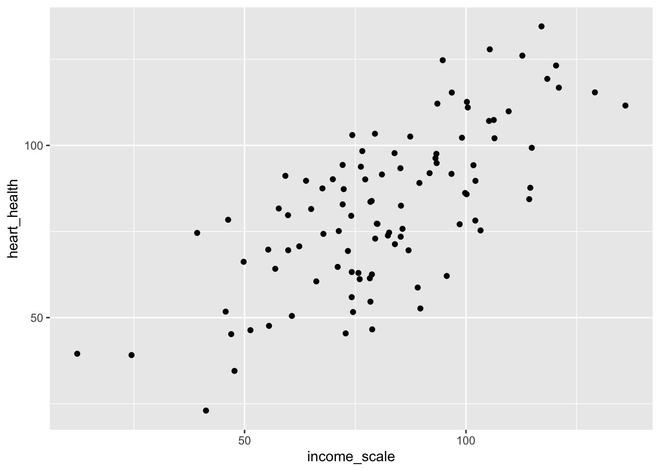
# visualdf_confound |>ggplot(aes(x = income_scale, y = heart_health)) +geom_point()
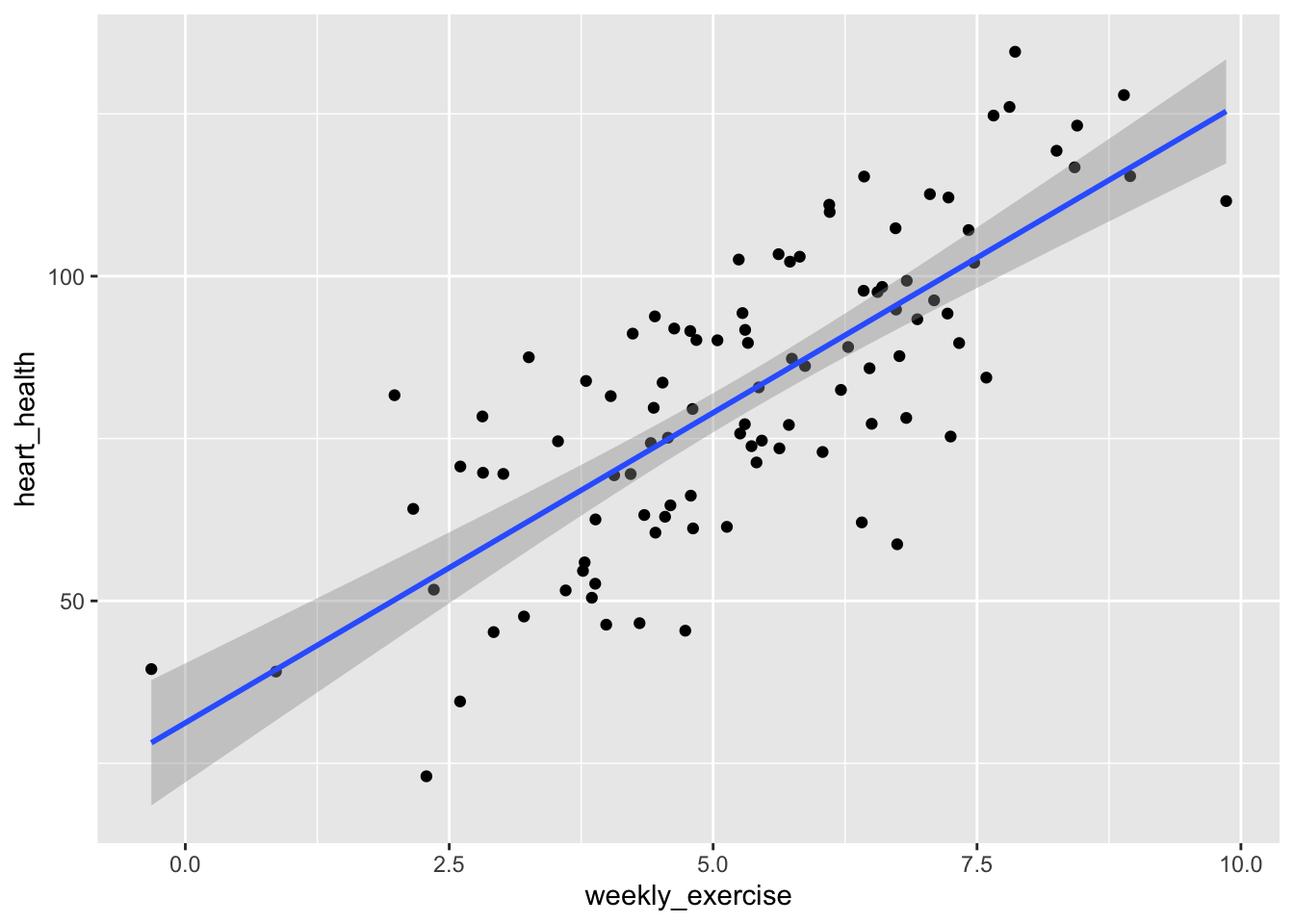
Okay! There is something wrong with this model, yes? We know income scale doesn’t actually impact heart health; rather, this is done through weekly exercise! To take this into account we can do the following:
Call:
lm(formula = heart_health ~ weekly_exercise + income_scale +
    age + female, data = df_confound)

Residuals:
     Min       1Q   Median       3Q      Max
-24.8789  -7.5206  -0.6986   7.2529  25.7713

Coefficients:
                Estimate Std. Error t value Pr(>|t|)
(Intercept)     61.75064    5.56561  11.095  < 2e-16 ***
weekly_exercise  9.62967    1.34813   7.143 1.84e-10 ***
income_scale     0.01537    0.11096   0.139     0.89
age             -1.01886    0.10584  -9.626 1.04e-15 ***
female           9.36947    2.29096   4.090 9.04e-05 ***
---
Signif. codes:  0 '***' 0.001 '**' 0.01 '*' 0.05 '.' 0.1 ' ' 1

Residual standard error: 10.71 on 95 degrees of freedom
Multiple R-squared:  0.7918,    Adjusted R-squared:  0.783
F-statistic: 90.32 on 4 and 95 DF,  p-value: < 2.2e-16
df_confound |>ggplot(aes(x=weekly_exercise,y = heart_health)) +geom_point()+# let's add a line based on using a linear regressiongeom_smooth(method ="lm")
`geom_smooth()` using formula = 'y ~ x'
Now, income is no longer correlated!
Class Examples
Who Trades? 🚢
Fit a model that estimates how much a country exports, using a treatment variable of your choosing. Interpret the model output.
Use the dataset trade in the package juanr
Identify your y (outcome) and x (explanatory) variables
Use the lm() function to fit a model
Use tidy() to show the outcomes of the model
To use tidy() use the broom package
library(juanr)library(tidyverse)library(broom)?tradetrade_ols <-lm(exports ~ sum_igos, data = trade)tidy(trade_ols)
Do happier people tend to have more or fewer kids than less happy people? Regress childs (outcome) against happy (treatment). Interpret the output.
How does religion affect family size? Regress the number of siblings sibs (outcome) against respondent religion relig. Based on the output: which religion has the largest families, on average?
library(socviz)?gss_smgss_sm |>distinct(happy)
# A tibble: 4 × 1
  happy
  <fct>
1 Pretty Happy
2 Very Happy
3 <NA>
4 Not Too Happy