Extra Materials: Sampling, Bootstrapping, and Prediction

# load libraries
library(socviz)
library(juanr)
library(gapminder)
library(patchwork)
library(broom)
library(paletteer)
library(moderndive)

Sampling in R

Now imagine that instead of having data on every American, we only have a sample of 10 Americans. Why do we have a sample? Because interviewing every American is prohibitively costly. The same way a poll works: a sample is used to estimate American public opinion.

We can pick one sample of 10 people from gss_sm using the rep_sample_n() function from moderndive:

gss_sm %>% rep_sample_n(size = 10, reps = 1)

# A tibble: 10 × 33
# Groups:   replicate [1]
   replicate  year    id ballot       age childs sibs  degree race  sex   region
       <int> <dbl> <dbl> <labelled> <dbl>  <dbl> <lab> <fct>  <fct> <fct> <fct> 
 1         1  2016  2409 2             66      7 11    High … Black Fema… Pacif…
 2         1  2016  2610 2             47      4  1    High … White Fema… W. So…
 3         1  2016   512 1             68      2  2    Bache… White Fema… New E…
 4         1  2016  1097 3             39      0  1    High … White Male  W. No…
 5         1  2016  1917 1             47      0  2    Gradu… Black Fema… E. So…
 6         1  2016   241 2             37      5  2    High … Other Male  Pacif…
 7         1  2016  1458 3             30      0  2    High … White Fema… Mount…
 8         1  2016  1085 1             39      1  3    Lt Hi… White Male  W. No…
 9         1  2016  1557 3             64      0  1    High … White Fema… Middl…
10         1  2016   316 2             66      4  2    High … White Male  E. No…
# ℹ 22 more variables: income16 <fct>, relig <fct>, marital <fct>, padeg <fct>,
#   madeg <fct>, partyid <fct>, polviews <fct>, happy <fct>, partners <fct>,
#   grass <fct>, zodiac <fct>, pres12 <labelled>, wtssall <dbl>,
#   income_rc <fct>, agegrp <fct>, ageq <fct>, siblings <fct>, kids <fct>,
#   religion <fct>, bigregion <fct>, partners_rc <fct>, obama <dbl>

Note

size = size of the sample; reps = number of samples

We can then calculate the average number of kids among that sample of 10 people.

gss_sm %>% rep_sample_n(size = 10, reps = 1) %>% 
  summarise(avg_kids = mean(childs, na.rm = TRUE))

# A tibble: 1 × 2
  replicate avg_kids
      <int>    <dbl>
1         1      1.8

This is our sample estimate of the population parameter.

How to simulate

If we take lots of samples of size 20 \(\rightarrow\) uncertainty in a sample of 20.

gss_sm %>%
  rep_sample_n(size = 20, reps = 1000)

If we take lots of samples of size 100 \(\rightarrow\) uncertainty in a sample of 100:

gss_sm %>%
  rep_sample_n(size = 100, reps = 1000)

So to see how uncertain we should feel about gss_sm, we should take many samples that are the same size as gss_sm:

gss_sm %>% 
  rep_sample_n(size = 2867, reps = 1000)

Note

nrow(DATA) tells you how many observations in data object

If we have a dataset of 2,867 observations and ask R to randomly pick 2,867 observations, we’ll just get a bunch of copies of the original dataset:

gss_sm %>% 
  rep_sample_n(size = nrow(gss_sm), reps = 1000)

Solution: sample with replacement \(\rightarrow\) once we draw an observation it goes back into the dataset, and can be sampled again!

gss_sm %>% 
  rep_sample_n(size = nrow(gss_sm), reps = 1000, replace = TRUE)

Sampling with and without replacement

If we were sampling 4 of these delicious fruits:

fruits = c("Mango", "Pineapple", "Banana", "Blackberry")
fruits

[1] "Mango"      "Pineapple"  "Banana"     "Blackberry"

It would look like this, with and without replacement:

Sample, no replace	Mango	Banana	Pineapple	Blackberry
Sample, replace	Pineapple	Pineapple	Banana	Blackberry

Example: Polling Crime Victimization

library(juanr)

data <- crime |>
  filter(pais == "Mexico")

boot_data = data |> 
  rep_sample_n(size = nrow(data), reps = 1000, replace = TRUE) |> 
  summarise(avg = mean(vic1ext, na.rm = TRUE),
            standard_error = sd(vic1ext, na.rm = TRUE)) |>
  mutate(low = avg - 1.96 * standard_error, 
         high = avg + 1.96 * standard_error) 

ggplot(boot_data, aes(x = avg)) + 
  geom_histogram(fill = red, color = "white") + 
  theme_nice() + 
  labs(x = "Average number of Individuals who are Victims of a Crime in Mexico") +
  annotate(geom = "rect", 
           xmin = quantile(boot_data$avg, probs = c(.025)), 
           xmax = quantile(boot_data$avg, probs = c(.975)), 
           ymin = 0, ymax = Inf, 
           alpha = .5, fill = yellow)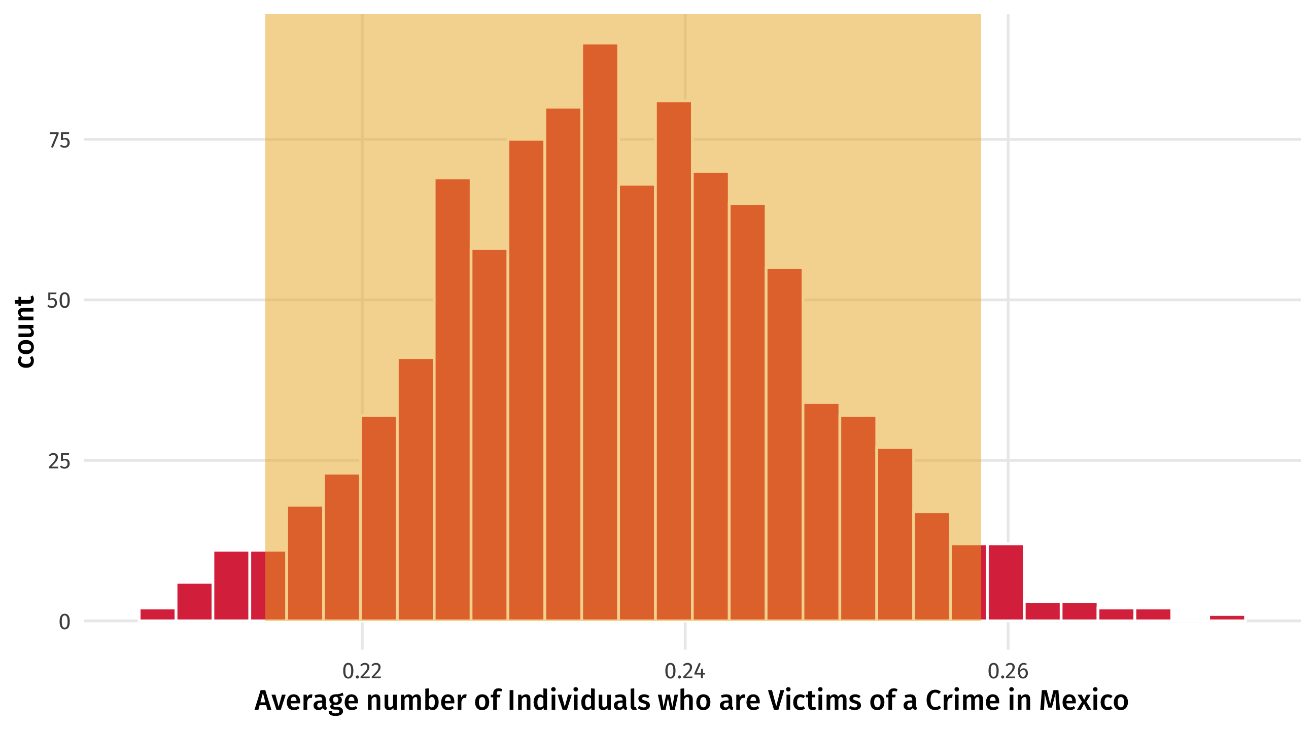

Bootstrapping Regression

We can simulate uncertainty in our estimate by bootstrapping

boot_lm_kids = gss_sm %>% 
  rep_sample_n(size = nrow(gss_sm), reps = 1000, replace = TRUE) %>% 
  nest(data = -replicate) %>% 
  mutate(model = data %>% map(.x = ., .f = ~lm(childs ~ age, data = .x))) %>% 
  mutate(results = map(model, tidy)) %>% 
  unnest(results) %>% 
  ungroup() %>% 
  filter(term == "age") 

boot_lm_kids %>% 
  select(`Bootstrap` = replicate, `Coefficient` = term, Estimate = estimate) %>%
  slice(1:10) %>% 
  knitr::kable(digits = 4)

Bootstrap	Coefficient	Estimate
1	age	0.0345
2	age	0.0336
3	age	0.0361
4	age	0.0319
5	age	0.0379
6	age	0.0360
7	age	0.0344
8	age	0.0339
9	age	0.0356
10	age	0.0352

How much might our estimate of lm(childs ~ age) vary? Look at the standard error

# A tibble: 1 × 2
    mean standard_error
   <dbl>          <dbl>
1 0.0346        0.00165

You might report it as .0345, +/- 2 standard errors.

We can also look at the 95% confidence interval – we are 95% “confident” that the true effect of age on the number of children a person has falls within this range. lm() will estimate the standard error of regression estimates for us using the statistical theory approach, but the results are similar to bootstrapping.

mod = lm(obama ~ sex, data = gss_sm)
tidy(mod)

# A tibble: 2 × 5
  term        estimate std.error statistic   p.value
  <chr>          <dbl>     <dbl>     <dbl>     <dbl>
1 (Intercept)   0.576     0.0177     32.6  5.84e-182
2 sexFemale     0.0871    0.0234      3.72 2.06e-  4

We can also ask tidy for the 95% CI:

tidy(mod, conf.int = TRUE)

# A tibble: 2 × 7
  term        estimate std.error statistic   p.value conf.low conf.high
  <chr>          <dbl>     <dbl>     <dbl>     <dbl>    <dbl>     <dbl>
1 (Intercept)   0.576     0.0177     32.6  5.84e-182   0.541      0.611
2 sexFemale     0.0871    0.0234      3.72 2.06e-  4   0.0412     0.133

conf.low and conf.high are the lower and upper bound of the 95% CI

Prediction (by hand)

weight_model = lm(mpg ~ wt, data = mtcars)

The equation for the model is:

\(\widehat{mpg} = 37.29 - 5.34(wt)\)

We only have one explanatory variable to work with (wt), so our scenario can only rely on weight

Scenario: a car that weighs 3.25 tons \(\rightarrow\) what fuel efficiency should we expect?

To get an estimate of mpg, we simply plug in the value of “weight” we are interested in:

Estimate for weight = 3.25

\(\widehat{mpg} = 37.29 - 5.34 \times \color{red}{3.25} = 19.935\)

Prediction (in R)

First define the scenario we want a prediction for, using crossing()

weight_scenario = crossing(wt = 3.25) 
weight_scenario

# A tibble: 1 × 1
     wt
  <dbl>
1  3.25

Note

the variables in crossing have to have the same name as the variables in the model

We can then combine our scenario with our model using augment()

augment(weight_model, newdata = weight_scenario)

# A tibble: 1 × 2
     wt .fitted
  <dbl>   <dbl>
1  3.25    19.9

augment takes the values for our scenario and plugs them into our model equation to get an estimate

Note

We tell augment what our new scenario is using the newdata = argument

We can also look at multiple scenarios, maybe a light, medium, and heavy car:

weight_scenario = crossing(wt = c(1.5, 3, 5)) 
weight_scenario

# A tibble: 3 × 1
     wt
  <dbl>
1   1.5
2   3  
3   5  

And then use augment to get the estimates:

augment(weight_model, newdata = weight_scenario)

# A tibble: 3 × 2
     wt .fitted
  <dbl>   <dbl>
1   1.5    29.3
2   3      21.3
3   5      10.6

Sequence of scenarios

Or we can look at a sequence of scenarios using the seq() function

Example: estimates for every weight between 2 and 6 tons, in .1 ton increments

seq_weights = crossing(wt = seq(from = 2, to = 6, by = .1)) 
seq_weights

# A tibble: 41 × 1
      wt
   <dbl>
 1   2  
 2   2.1
 3   2.2
 4   2.3
 5   2.4
 6   2.5
 7   2.6
 8   2.7
 9   2.8
10   2.9
# ℹ 31 more rows

Note

seq needs a starting point (from), an end point (to), and an interval (by)

And then get predictions for all these scenarios:

augment(weight_model, newdata = seq_weights)

# A tibble: 41 × 2
      wt .fitted
   <dbl>   <dbl>
 1   2      26.6
 2   2.1    26.1
 3   2.2    25.5
 4   2.3    25.0
 5   2.4    24.5
 6   2.5    23.9
 7   2.6    23.4
 8   2.7    22.9
 9   2.8    22.3
10   2.9    21.8
# ℹ 31 more rows

Multiple Regression

big_model = lm(mpg ~ wt + cyl + hp + am, data = mtcars)

big_scenario = crossing(wt = 3, cyl = 4, hp = 120, am = 1)

augment(big_model, newdata = big_scenario)

# A tibble: 1 × 5
     wt   cyl    hp    am .fitted
  <dbl> <dbl> <dbl> <dbl>   <dbl>
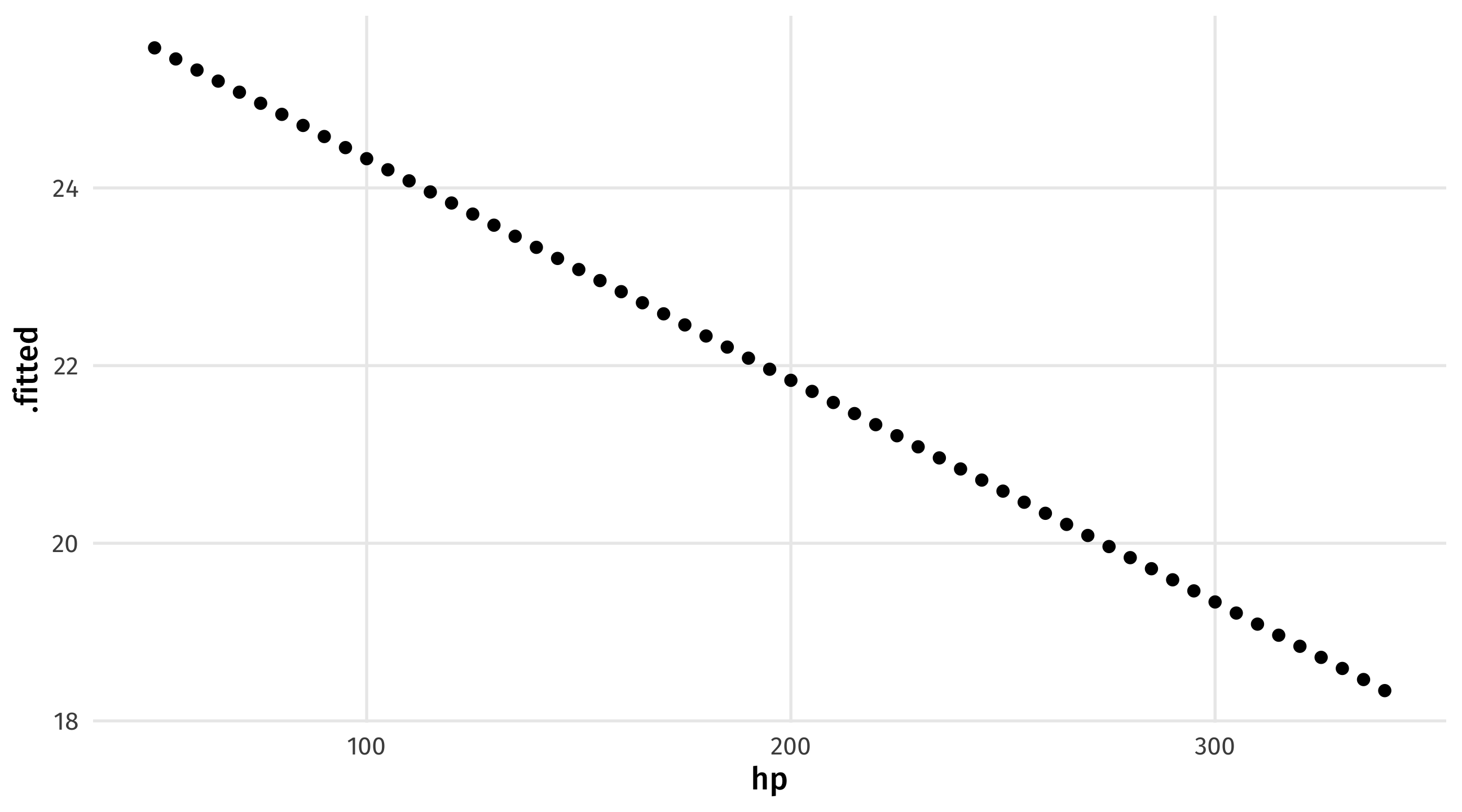
1     3     4   120     1    23.8

We can use seq() to see what happens when horsepower changes while everything else is left at a fixed value

varying_hp = crossing(wt = 3, cyl = 4, am = 1, hp = seq(from = 50, to = 340, by = 5))

augment(big_model, newdata = varying_hp)

# A tibble: 59 × 5
      wt   cyl    am    hp .fitted
   <dbl> <dbl> <dbl> <dbl>   <dbl>
 1     3     4     1    50    25.6
 2     3     4     1    55    25.5
 3     3     4     1    60    25.3
 4     3     4     1    65    25.2
 5     3     4     1    70    25.1
 6     3     4     1    75    25.0
 7     3     4     1    80    24.8
 8     3     4     1    85    24.7
 9     3     4     1    90    24.6
10     3     4     1    95    24.5
# ℹ 49 more rows

Visualizing predictions

We could then store our estimate, and use it for plotting

hp_pred = augment(big_model, newdata = varying_hp)
ggplot(hp_pred, aes(x = hp, y = .fitted)) + geom_point()